MathPad guide
The guide that comes with the app (Help > Guide), every topic of it. The math in the tables and the small notebooks was typed and worked out by MathPad itself as this page was made. Keys are shown as on a Mac: on Windows, Ctrl takes the place of Cmd and Alt of Option.
Start here
Getting Started
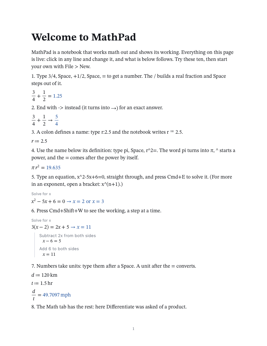
MathPad is a notebook that works math out. You write a problem the way you would on paper, in real fractions, roots and powers, and the notebook gives the answer, with the working step by step when you ask for it.
Regions
A notebook is a column of regions that run down the pages. There are three kinds:
- Math: one line of math that is worked out. A new notebook starts with an empty one.
- Text: a paragraph, a heading or a note.
- Plot: a graph of one or more expressions.
Enter in a math region starts a new math region below. In an empty math region, a quote mark " or Space typed first turns it into a text region, so you can simply start writing. The Home tab's Math, Text and Plot buttons do the same (Cmd+Shift+M, Cmd+Shift+T, Cmd+Option+G).
The notebook is worked out from the top down: a name defined in one region is known in every region below it, and in none above.
A first problem
Click in the empty region and type
| Type | You get | |
|---|---|---|
| x^2-5x+6=0 |  | An equation. ^ starts the power, and the - that follows it is typed after the power, not in it. |
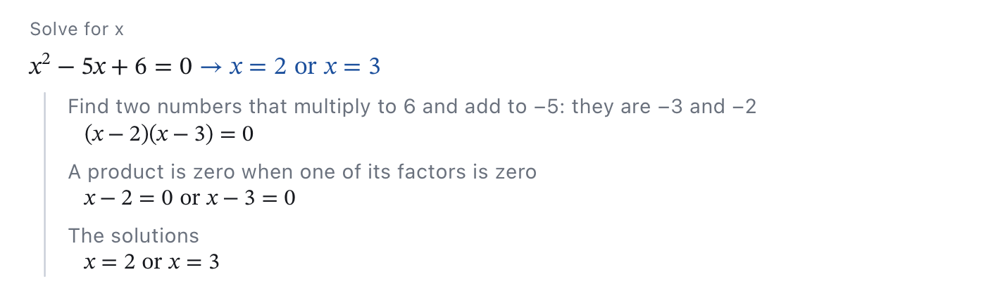
Now ask for the solution: press Cmd+E, or choose Solve on the Home tab. The answer appears after an arrow. Press Cmd+Shift+W (Show Steps) to see how it was found:
Asking for a number
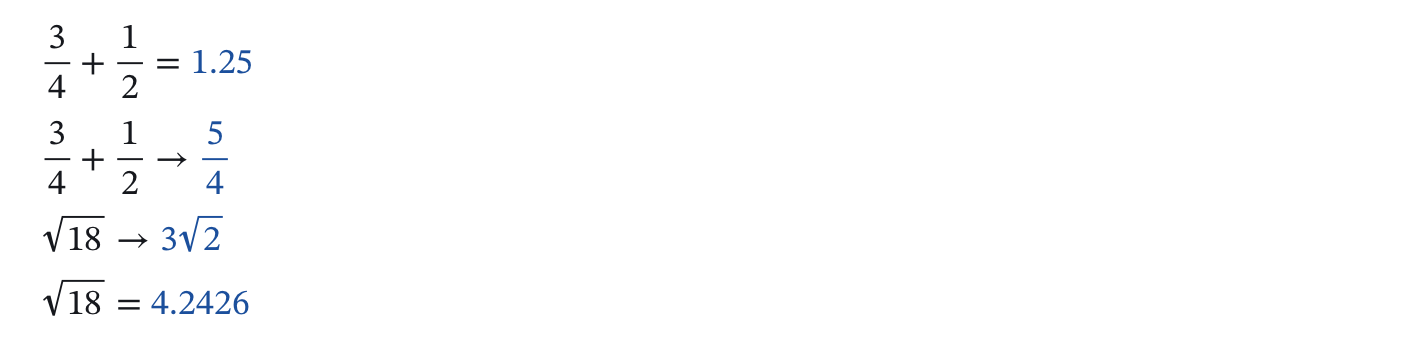
End a line with = and the notebook writes the number after it. End it with -> (which turns into →) for an exact answer in symbols.
Where to go next
- Typing Math has every key.
- Defining and Evaluating is about names,
=and →. - Solving and Working lists what can be asked of a region.
- Help > Examples has ready-made notebooks to change and learn from; the welcome notebook is ten lines to try.
Typing Math
Math is typed on one line of keys and builds itself into two dimensions as you go. The middle column below is what the keys at the left really make: it was typed into the editor when this page was put together.
Fractions, powers and roots
| Type | You get | |
|---|---|---|
| 1/2 | 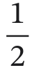 | / makes a fraction of what stands left of the caret and goes to the bottom. |
| 1/2Space+3 | 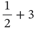 | Space steps out of the fraction (or of any structure). |
| a/b+c | 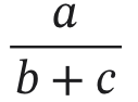 | Without the Space you are still in the bottom. |
| (a+b)/c | 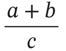 | A bracket and what is in it goes on top as a whole. |
| sin(x)/x | 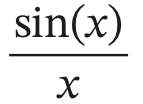 | So does a function with its bracket. |
| x^2+1 | 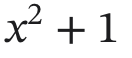 | ^ starts a power. A simple power (one number or one name) is left by typing on: the + comes after it. |
| x^2/3 | 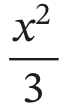 | The same with /: the power goes on top with its base. |
| e^x= |  | And with =, a comma or a closing bracket. |
| x^-1+2 | 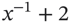 | A - typed first in the exponent stays: a negative power. |
| x^(n+1)+2 | 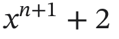 | For more in the exponent, open a bracket. It is taken away again when you type on after closing it. |
| e^2xSpace+1 | 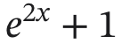 | Letters and digits stay in the exponent; Space (or Right) always steps out. |
| e^-x^2 |  | A power in a power. |
| sin^2(x)+cos^2(x) |  | The square of a function: the bracket after the power is the function's. |
| \2 |  | \ is a square root. |
| \x+1Space-3 | 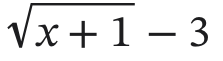 | Space steps out of the root. |
| Insert > Nth Root3Tab8 |  | An n-th root comes from Insert > Nth Root: the degree first, then Tab. |
Names, subscripts and indexes
| Type | You get | |
|---|---|---|
| area |  | Letters side by side are one name. |
| 2x |  | A number before a name multiplies. |
| xSpacey |  | A Space between two names parts them: x times y. |
| x_1+x_2 | 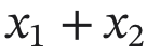 | _ right after a name starts a subscript that is part of the name. Like a simple power, it is left by typing on. |
| F_max | 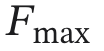 | The name is F_max. |
| v[2 |  | [ right after a name is an index: the second entry of v. |
| v[i+1]-v[i] | 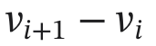 | An index is closed with ], so sums can be typed in it. |
| M[1,2 | 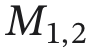 | Row 1, column 2 of a matrix. |
| [1,2,3 | 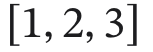 | [ anywhere else starts a list. |
| f(x) |  | A name followed by a bracket is a function of what is in it. |
| f'(x) | 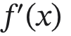 | An apostrophe is a prime: the derivative of f. |
Signs
| Type | You get | |
|---|---|---|
| a:5 | 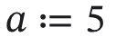 | : is ≔, which defines a name. |
| 2*3-1 | 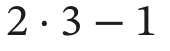 | * is the multiplication dot and - a true minus. |
| x<=5 | 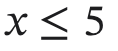 | < then =. |
| x>=5 | 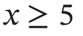 | > then =. |
| x<>y | 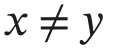 | < then > is ≠. (Right after a name or a number ! is a factorial, so 5!= asks for 120.) |
| f(x)-> | 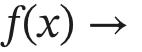 | - then > is →: work this out in symbols. |
| 1..5 |  | Two points are a range. |
| |x-1|+2 | 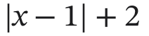 | | opens an absolute value and, at its end, closes it. |
| n! |  | A factorial. |
| s:"hello | 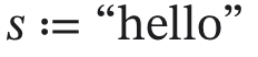 | A quote mark in math starts a piece of text (a string); a second one ends it. |
Greek letters and constants
Spell a Greek letter out and it turns into the letter as soon as the next thing typed isn't a letter. The Insert tab has them too.
| Type | You get | |
|---|---|---|
| alpha+betaSpace | 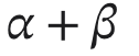 | Small letters by their names; the letter appears when the next key isn't a letter. |
| OmegaSpace |  | A capital for the capital. |
| 2piSpacer |  | π is pi; the Space parts it from the r. |
| infSpace |  | Infinity. |
| e^x |  | The letter e is the base of natural logarithms. |
| 2i+3 | 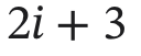 | An i or a j right after a number is the imaginary unit. |
A word inside a longer name is left alone: pivot stays pivot.
Templates
Sums, integrals, derivatives, limits, cases, programs and matrices come from the Insert tab (or Insert menu). The caret starts in the first place to fill; Tab goes to the next empty place and Shift+Tab back.
| Type | You get | |
|---|---|---|
| Ctrl+M1Tab2Tab3Tab4 | 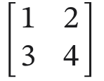 | A matrix: Tab goes from cell to cell. |
| Cmd+Shift+UkTab1TabnTabk^2 | 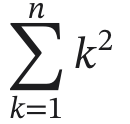 | A sum: the variable, where it starts, where it ends, then what is added. |
| Insert > Definite Integral0Tab2Tabx^2Tabx | 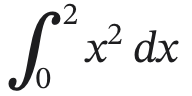 | A definite integral: the limits, the integrand, the variable. |
| Cmd+Shift+Ix^2Tabx | 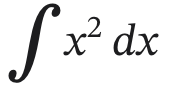 | An integral without limits. |
| Cmd+Shift+DxTabx^3 | 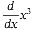 | A derivative: the variable first. |
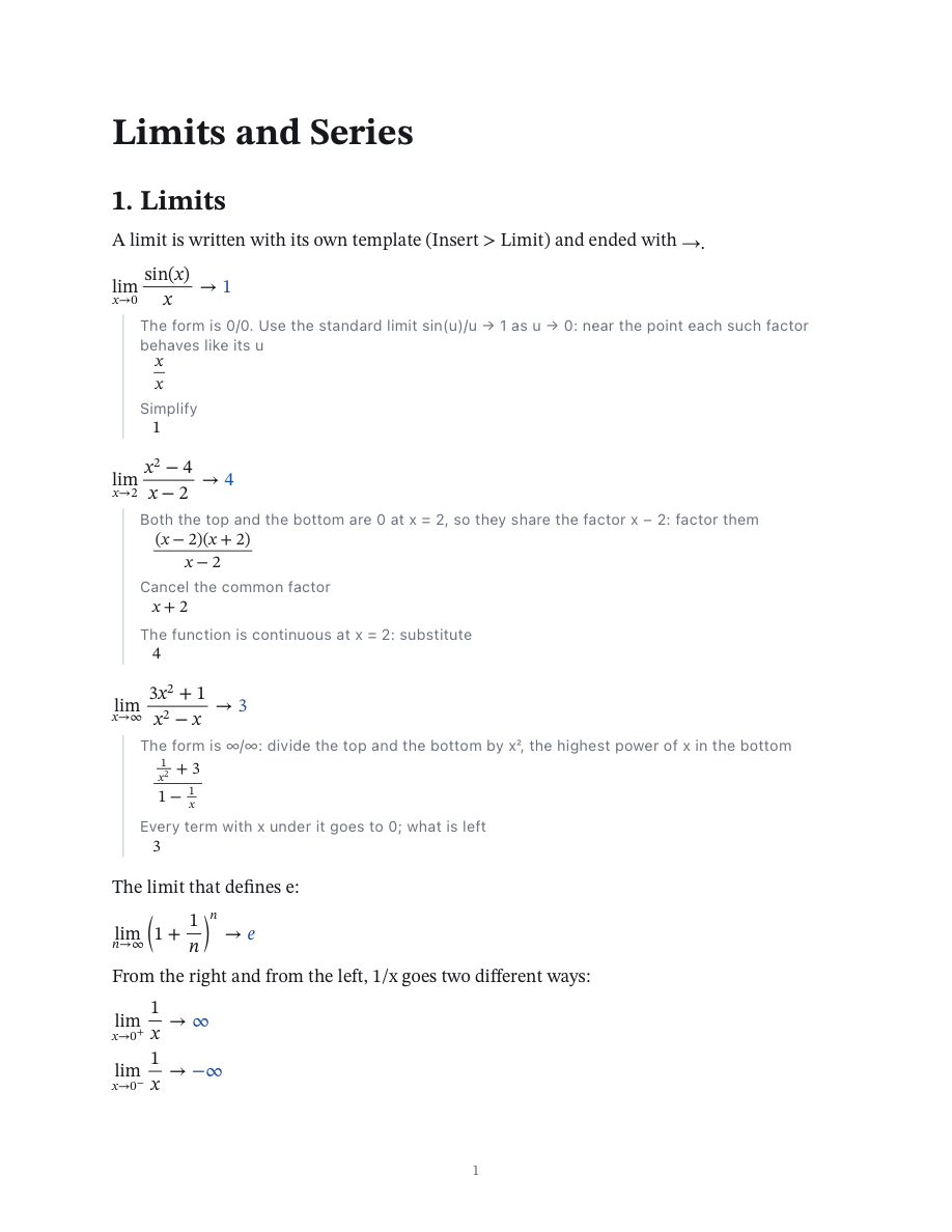
| Insert > LimitxTab0Tabsin(x)/x | 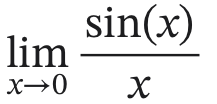 | A limit: the variable, what it approaches, the expression. |
| f(x):Insert > Cases-xTabx<0Tabx | 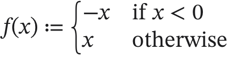 | Cases: a value, its condition, the next value. An empty last condition means otherwise. |
Moving and deleting
| Key | What it does |
|---|---|
Left, Right | One place at a time, into and out of fractions, powers and roots. |
Up, Down | Between the top and bottom of a fraction, the limits of a sum, the rows of a matrix, the lines of a program; otherwise to the region above or below. |
Space | Out of the structure the caret is in, to its right. (Inside brackets, between a name and what follows it, it parts the two instead: a product.) |
+ - * / = < > , ; : ) | At the end of a power or a subscript that holds one number or one name: out of it first, then the sign. |
Tab, Shift+Tab | The next, or the last, empty place. |
Home, End | The ends of the row, then of the whole region. |
Shift + an arrow | Selects. A structure is selected as a whole. |
Backspace | Deletes a character; after a structure it first selects it, and a second press deletes it. At the start of a bottom, a power or a root it takes the structure away and keeps what was in it. |
Enter | A new math region below; in a program a new line, in a matrix the cell below, in a plot's line a new trace. |
With something selected, / puts it on top of a fraction, ^ raises it to a power, \ puts it under a root and ( wraps it in brackets.
Things to watch
1/2/3is 1 over 2/3. For a half of a third, step out first:1/2,Space,/3.- A power is left by typing on only while it is simple: after
e^2xa+comes after the power, but once there is a sign in the exponent (typed inside on purpose, with the caret moved back in) typing stays there untilSpaceorRight. For an exponent like n+1, typex^(n+1). x^2/3is x² over 3. For x to the two thirds, typex^(2/3).x^2(keeps the bracket in the exponent, unless the power is on a function's name (sin^2(x)).!right after a name or a number is a factorial, so5!=asks for 120. Not equal is typed<>.- In a plot's own line
Enterstarts another trace; in an empty one it ends the list and starts a math region under the plot. - A unit is typed after its number with a
Spacebetween (5,Space,m);5mand5*mare products. See Units.
Defining and Evaluating
Three signs say what a math region is for.
| Sign | Typed | What the region does |
|---|---|---|
| ≔ | : | Defines the name at its left. Nothing is shown. |
| = at the end | = | Shows the value as a number. |
| → at the end | -> | Shows the result in symbols: exact fractions, roots, π. |
An = with something on both sides is an equation, which can be solved.
Names

A definition is seen by every region below it. Change a and everything below that uses it follows. A name may be defined again further down; from there on the new value counts.
A name can be several letters (area), have a subscript (F_max, typed F_max) or be a Greek letter. The words of programs (if, else, for, while, return, break, continue, otherwise) can't be names.
Functions
A name with its variables in brackets defines a function.

Numbers or symbols
= always gives a number. → keeps things exact while Exact Results is on (Math tab), and works with names that have no value at all:
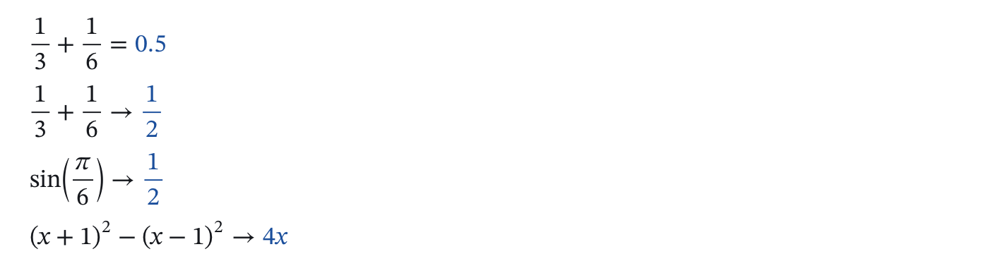
More Digits and Fewer Digits (Cmd+Shift+. and Cmd+Shift+,) set how many digits follow the point. Angles are in radians unless Degrees is on; a number written with deg is an angle in degrees either way.

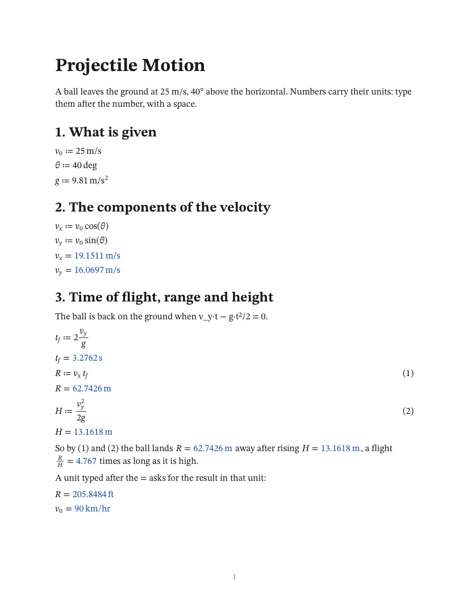
A unit after the =
A unit typed after the final = asks for the result in that unit. See Units.

Math in a sentence
In a text region, $ starts math inside the sentence (so does Ctrl+=, and Insert > Inline Math). Everything is typed there as in a math region, and a second $, Return, Esc or Right at its end goes back to the words. It is worked out where it stands, like a region of its own: : defines for everything after it, the rest of the sentence too, and a row ending in = or -> shows its result.

The arrows walk into the math and out of it; Backspace right after it selects it first and then deletes it. Selected text becomes math with $ (or Format > Region > Turn Selection into Math), and math becomes text again with Turn Math into Text. A dollar sign as itself is typed \$. What is wrong with math in a sentence is underlined in red, and the status bar says what while the caret is in it.
Numbered equations
Math > Number Equation (Cmd+Option+N) puts a number at the right margin of a math region; the numbers count down the notebook and follow when regions come and go. Name Equation gives the region a name, and Insert > Reference (Cmd+Option+R) lists the numbered equations and puts a reference to one into the sentence: it shows the equation's number, whatever that becomes. A double click on a reference, or a click with Cmd, goes to its equation.

When something is wrong
A region that can't be worked out says why in red under it, and the regions that depend on it say what they are missing.

Solving and Working
Besides = and →, a region can be asked something about the whole line, the way one would say it over a problem: solve this, simplify it, differentiate it. The Home tab has Solve; the Math tab and the Math menu have the common ones, the right-click menu offers what makes sense for the region under the mouse, and Ask (Cmd+Return) lists everything that can be asked of the line the caret is in.
| Ask | Keys | For |
|---|---|---|
| Solve | Cmd+E | An equation, an inequality or a system; an expression is solved where it is 0. |
| Solve in numbers | Ask | The roots as decimals, when there is no formula or it is too long to read. |
| Simplify | Cmd+Shift+Y | An expression or an equation. |
| Expand | Products and powers multiplied out. | |
| Factor | A polynomial as a product. | |
| Partial Fractions | A quotient of polynomials. | |
| Differentiate | The derivative with respect to a variable. | |
| Integrate | The antiderivative, or with limits the area. | |
| Limit | The limit as a variable goes to a point. | |
| Series | The Taylor series around a point. | |
| Tangent line | Ask | The line that touches a curve at a point. |
| Solve the differential equation, Find dy/dx | Ask | See Calculus. |
| Determinant, Inverse, Eigenvalues, … | Ask | For a matrix: see Matrices. |
| Evaluate | Cmd+Shift+N | A number. |
No Action takes the question away again. With several unknowns the first one is taken; the menus list the others (Solve for y).
Steps
Show Steps (Cmd+Shift+W) writes the working under the result, a line for each thing done, with the rule in words.
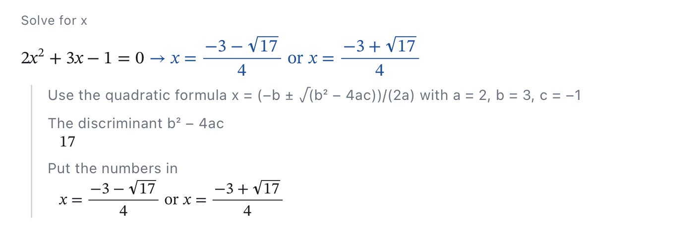
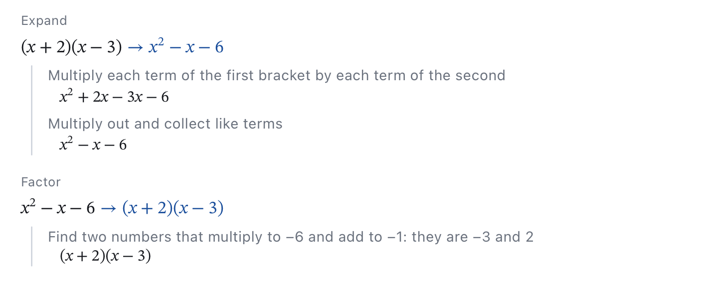
Systems
Write the equations as a list in square brackets and ask Solve. The equations needn't be linear: a circle and a line cross twice.
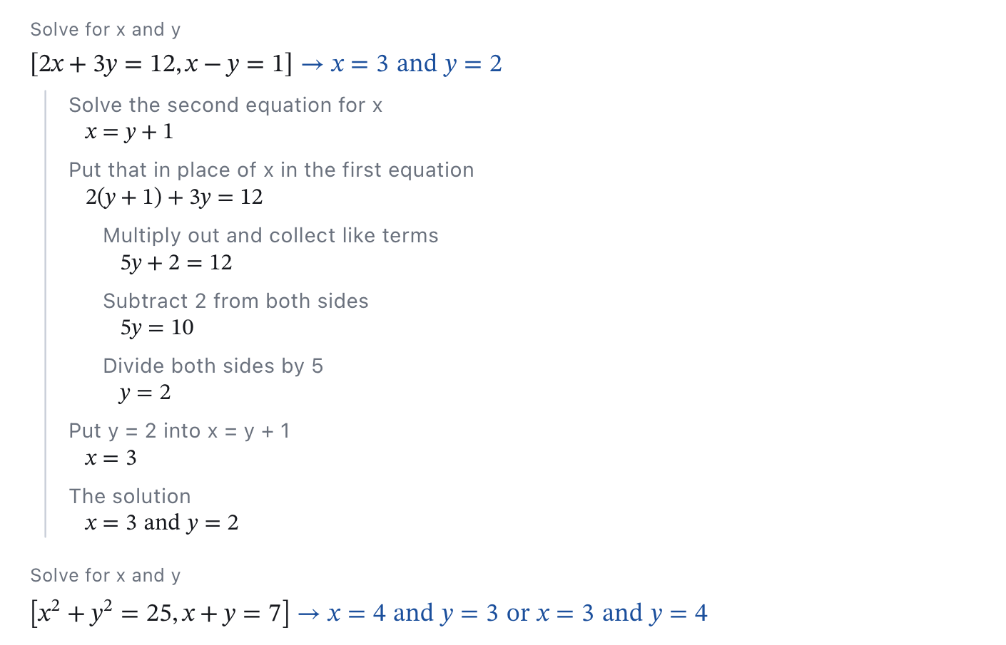
Inequalities and more
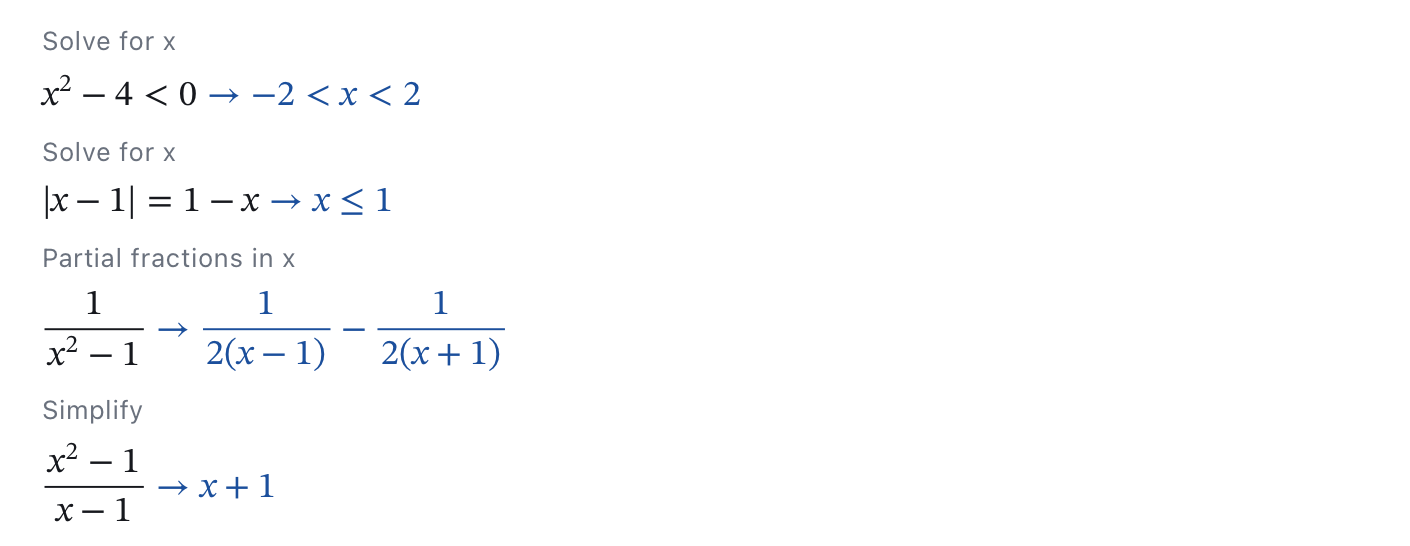
An answer can be a condition instead of a list of numbers: for an inequality, and for an equation that holds on a whole stretch.
Cubics, quartics, and when to ask for numbers
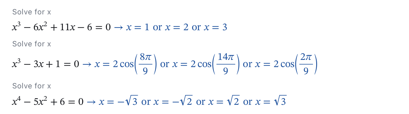
A cubic or a quartic that doesn't factor is solved by its formula. With three real roots a cubic's come as cosines (the only way to write them without ⅈ); a biquadratic comes in roots.
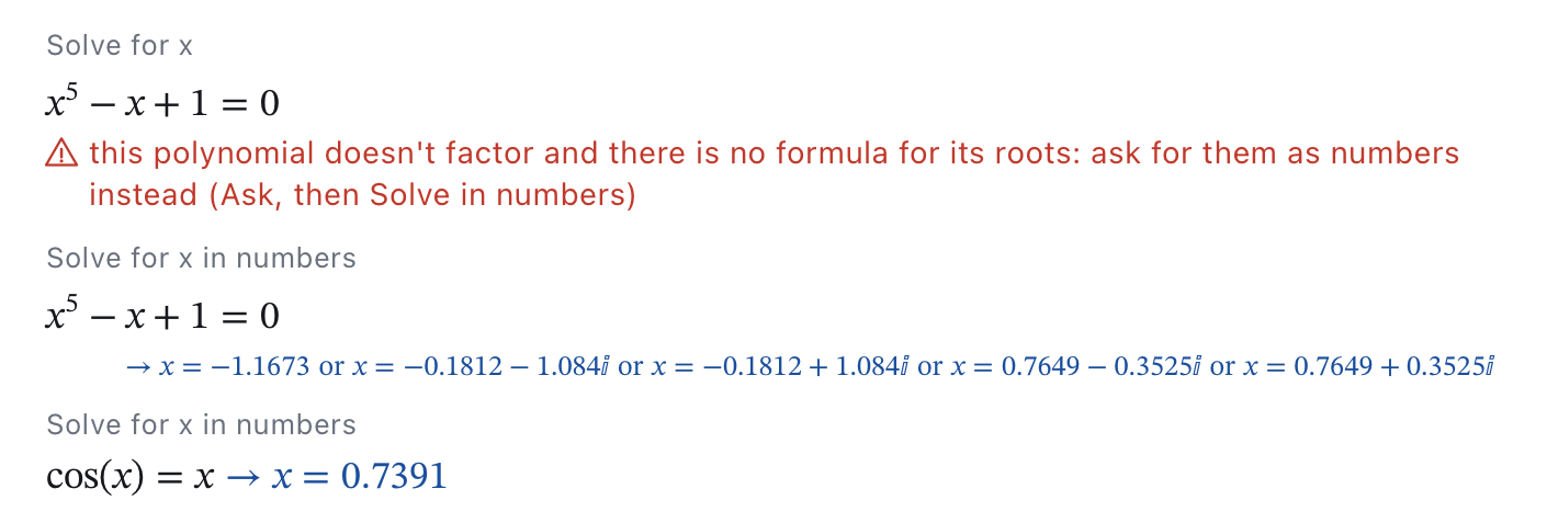
From the fifth degree on there is no formula, and some quartics have one too long to be of use. The region then says so, and Ask offers Solve for x in numbers first: every root of a polynomial, the complex ones too, and for other equations the places where the two sides cross.
Whole numbers of any size
With → whole numbers and fractions are exact however long they get; = gives the decimal.

As functions
Everything that can be asked can also be written out and ended with →, which is handy inside a longer line:
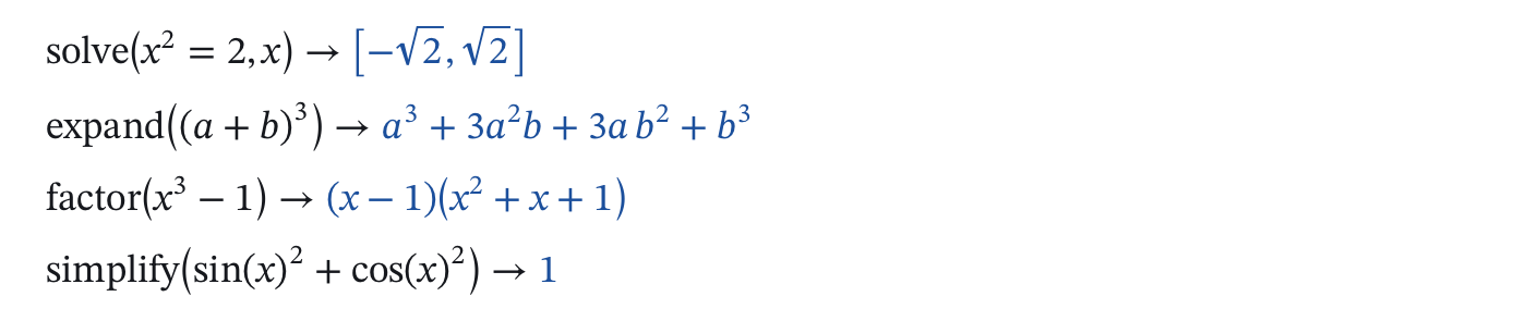
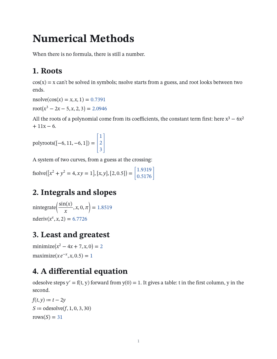
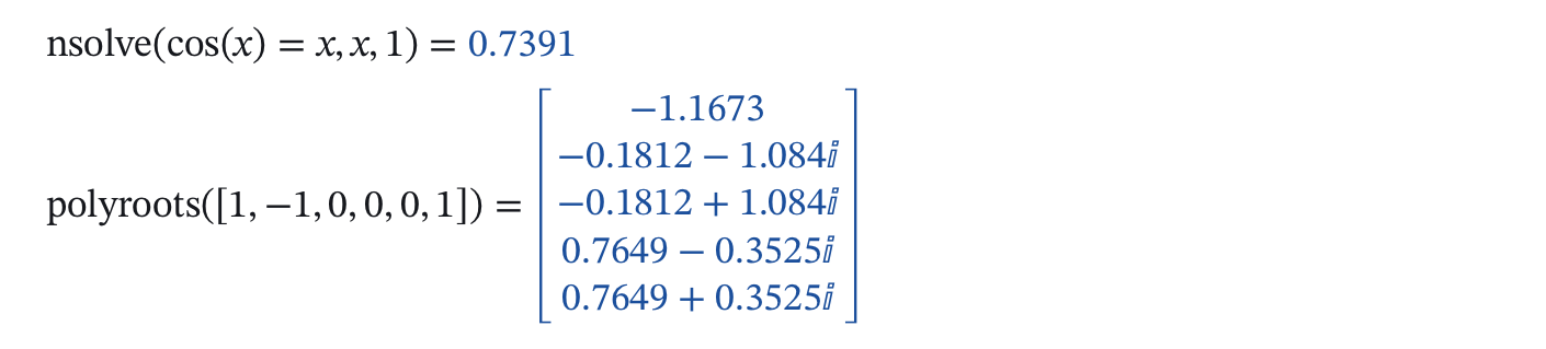
For numbers there are nsolve (one root, from a guess), root (between two ends) and polyroots (all the roots of a polynomial, from its coefficients with the constant term first):
Doing math
Units
A unit is written after a number, with a Space between: number, space, unit. Units multiply and divide, and the notebook keeps track of them.
| Type | You get | |
|---|---|---|
| 5Spacem |  | Five metres. The unit is upright. |
| 25Spacem/s | 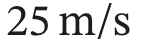 | A speed. After a unit / is a stroke on the line, the way results write it. |
| 9.81Spacem/s^2 | 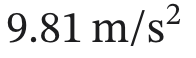 | An acceleration: ^ after a unit's name is its power. |
| 10SpaceW/(m*K) | 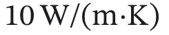 | Several units under the stroke go in a bracket; * is the dot. |
| 5Spacem/s/2 | 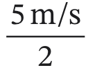 | What isn't a unit goes under a bar, the whole quantity above it. |
| F:20SpacekN | 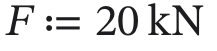 | A force with a name. |
| 5m |  | Without the space this is algebra: 5 times m, in italics. |
| 5*m | 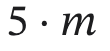 | And so is this, always. |
The space is what tells five metres from five times m. (With no m of your own, 5m still works out as five metres, since m then means nothing else; it just isn't written as a quantity.) Units are typed the way results, the palette and Quick Insert write them, on one line: 9.81 m/s². The same goes for a unit asked for after an = (v = km/h). For a unit stacked over a bar, select the top and type /, or take the fraction from the palette; both ways are read the same.
Results keep your units
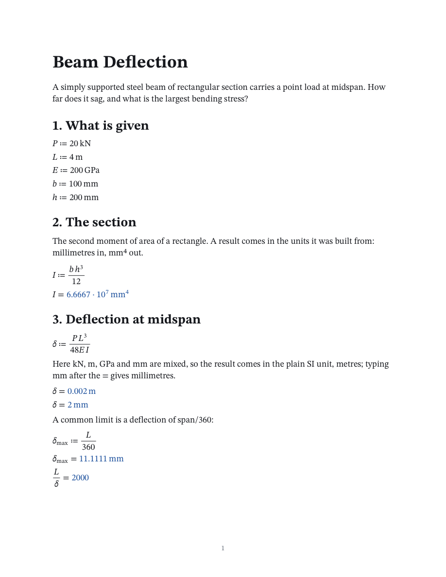
A result is shown in the units it was built from. What was given in kN and m comes back in kN·m, a distance in km over a time in h is a speed in km/h, and a number given in mm stays in mm.
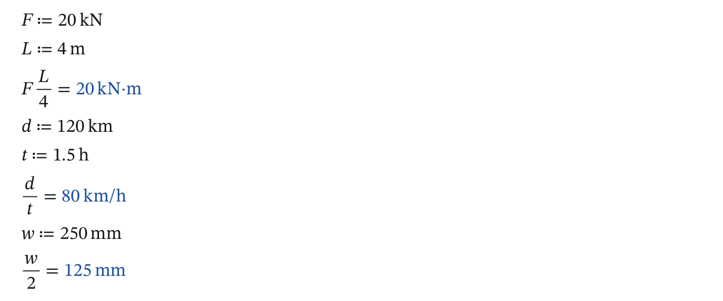
When the units a result was built from don't make one tidy unit, it goes to the named unit of its kind: kN over mm² is shown in MPa, V times A in W.
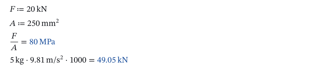
With nothing else to go by, a force, a pressure, a power, an energy, a voltage, a current or a resistance gets the prefix that reads best: 49050 N is written 49.05 kN. Lengths, masses and times are left in m, kg and s unless you gave them in something else: 0.5 m is not turned into 500 mm. Notebook Settings (Cmd+,) has the switch, Choose kN, MPa, kW… automatically.
Converting
A unit typed after the final = gives the result in that unit. Once the notebook has taken it for a unit, its letters stand upright.
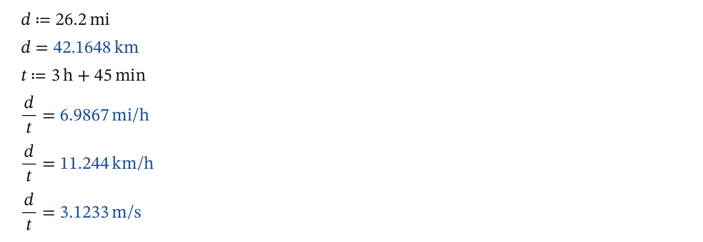
With US Customary Units on (Math menu), results that have nothing to say their unit come in feet, pounds and the like. Units that don't fit are an error, which is the point of carrying them:

A variable with a unit's name
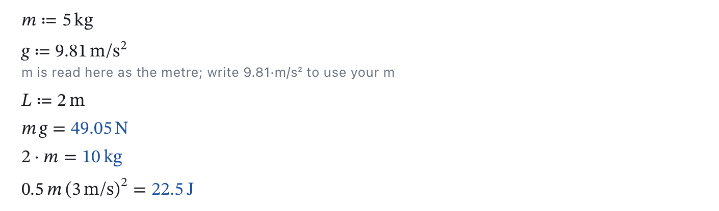
Every short unit is also a letter you may want for something else: m for a mass, s for a distance, t, h, g, A, V. You can define them; the notebook then reads each place by what stands there.
- By itself, right against a number, or after a dot, the name is yours:
m,2mand2·mmean your m from its definition down. - After a number and a space it is still the unit when it ends the product (
L ≔ 2 mis two metres) or stands with units that aren't names of yours (9.81 m/s²is an acceleration while s is nobody's variable). - With more factors after it, it is yours again:
0.5 m v²is half your mass times v².
The first time a name of yours is read as a unit, the region says so in small grey letters under it, with how to write it if you meant your own. The Variables panel marks such names also a unit.
Angles, temperatures and percent
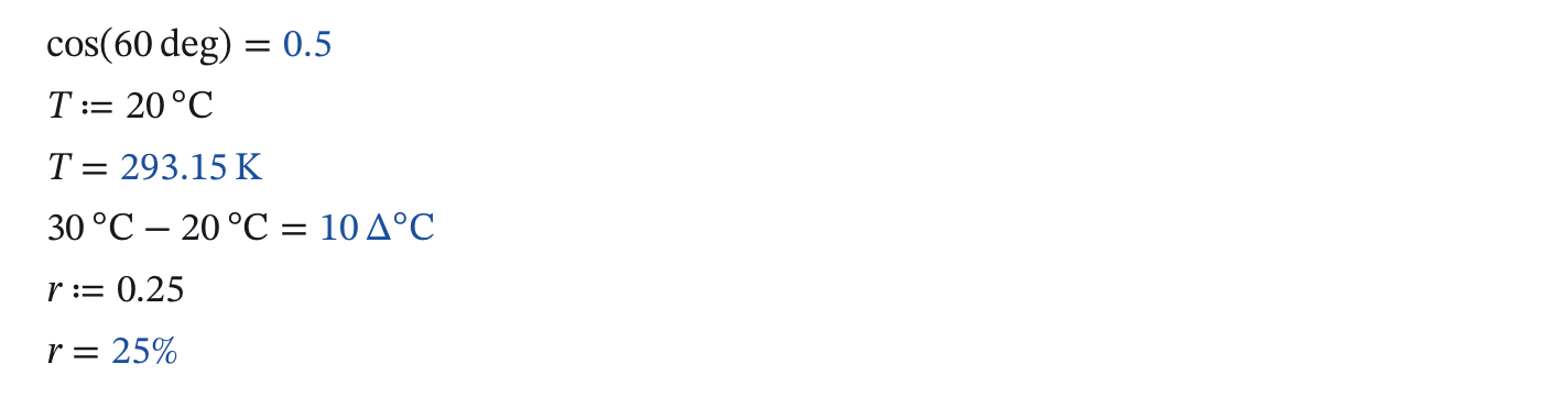
deg (or °) makes a number an angle in degrees whatever the notebook's setting, and an angle given in degrees is shown in degrees. °C and °F after a number are a temperature; the difference of two temperatures is in Δ°C, which is the size of a degree. A % after the final = shows a ratio as a percentage.
Things to watch
- The hour is
h(orhr), the minutemin, the inchinand the ohmohmor Ω. x = kmis read as asking for x in kilometres becausekmis a unit and x has a value.W = m gis an equation while W has no value.- A plot draws plain numbers: divide a quantity by its unit to plot it.
The Units Reference lists every unit.
Matrices
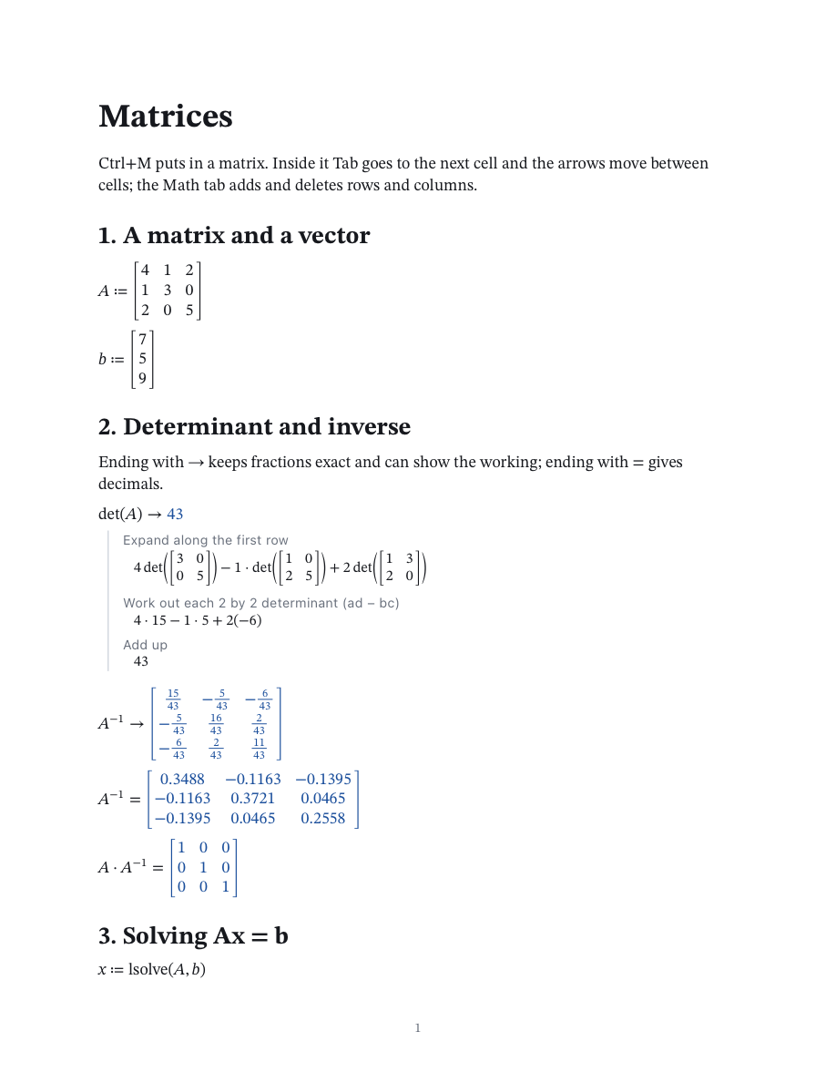
Ctrl+M puts in a 2 by 2 matrix (it is the Control key on a Mac too). Tab goes to the next cell, the arrows move between cells, and Enter goes down a column. The Math tab's Matrix group (and the Insert menu) adds and deletes rows and columns where the caret is.
| Type | You get | |
|---|---|---|
| A:Ctrl+M2Tab1Tab1Tab3 | 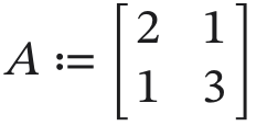 | A matrix with a name. |
| v:[1,2,3 | 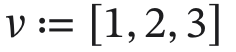 | A list in square brackets is a vector. |
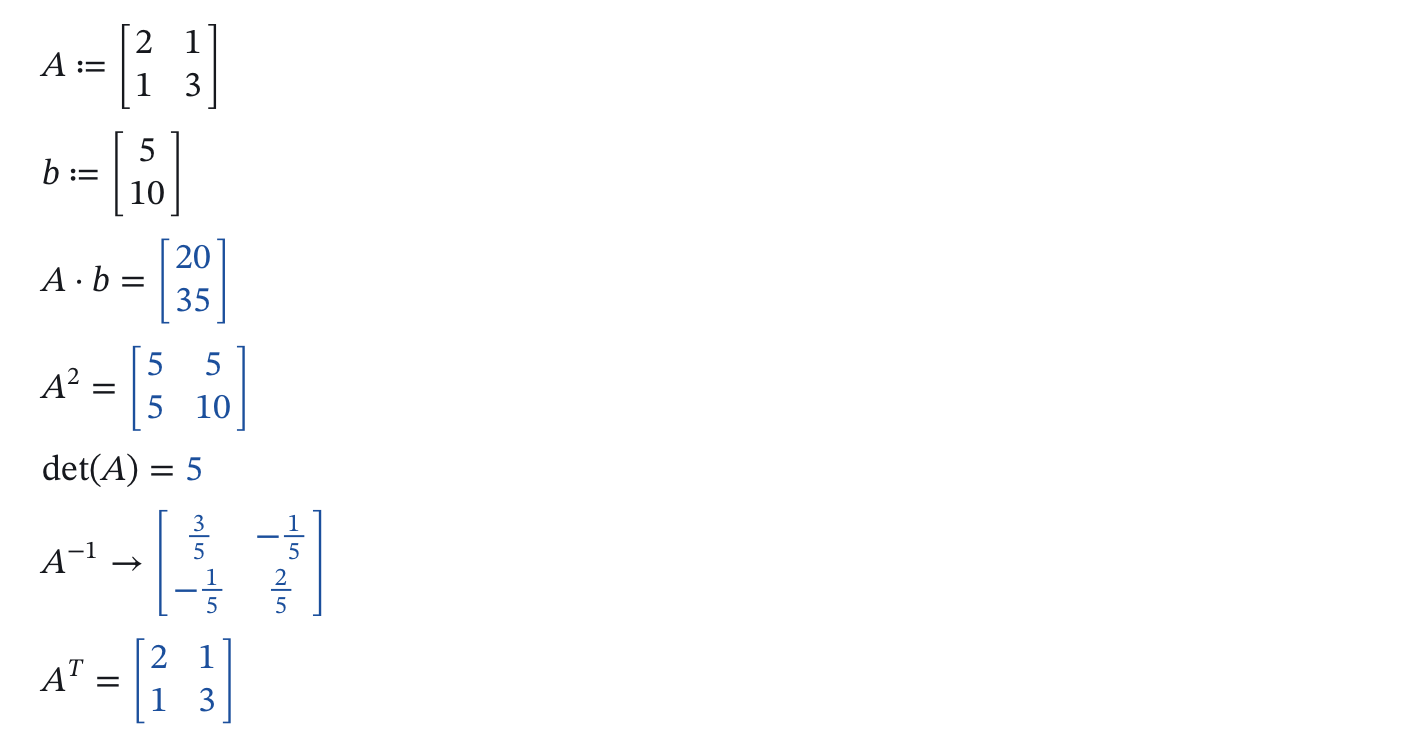
A power of −1 is the inverse and a power of T the transpose. → keeps the entries exact; = gives decimals.
Solving Ax = b
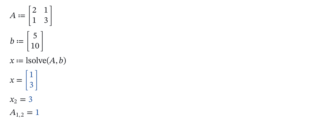
An index ([ right after the name) picks an entry; rows and columns are counted from 1.
Eigenvalues and the rest
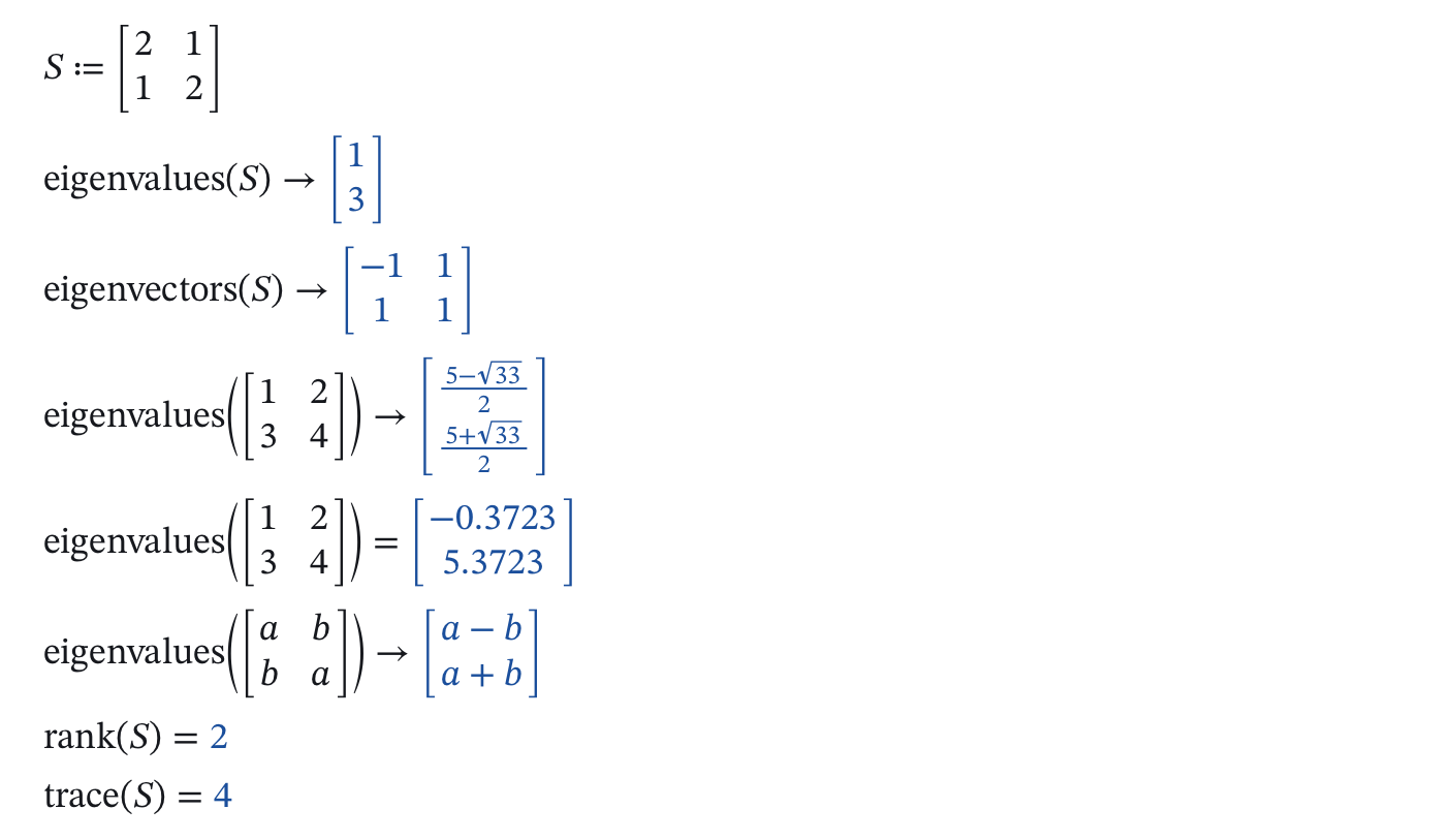
With → the eigenvalues of a small matrix are exact, in roots when they need them, and letters may stand in the matrix; = gives decimals for a matrix of any size. The eigenvectors are the columns of what eigenvectors gives, in the order of the eigenvalues.
Asking a matrix
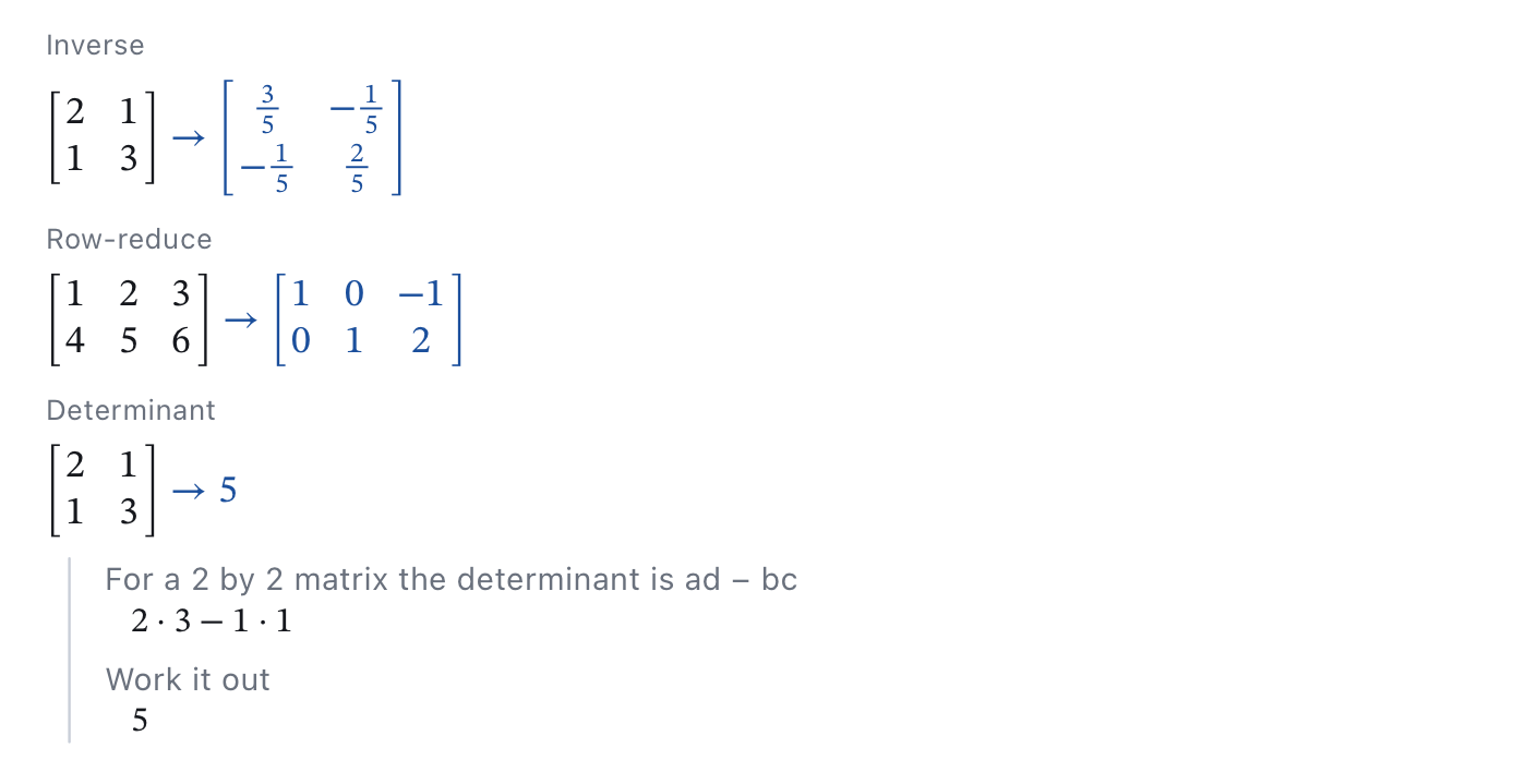
With the caret in a matrix (or in a line that is the name of one), Ask (Cmd+Return) offers Determinant, Inverse, Eigenvalues, Eigenvectors, Row-reduce and Transpose. The answer is worked in symbols, with its steps.
Vectors
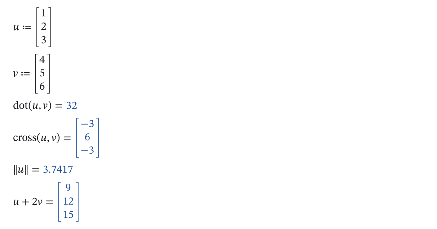
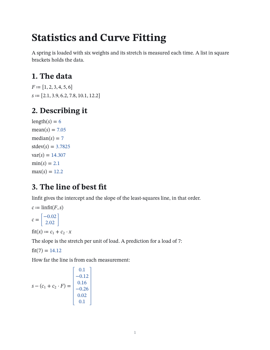
Lists work with the statistics functions (mean, stdev, sum, sort, …) and with arithmetic, entry by entry. The Functions Reference has every matrix function.
Calculus
Derivatives, integrals, limits, series and sums can be asked of an expression (Math tab), or written with their own signs from the Insert tab and ended with →. Either way Show Steps gives the working.
Derivatives
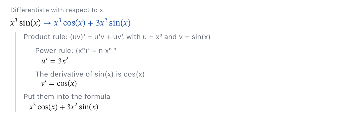
Written out (Cmd+Shift+D), and the second derivative from Insert > Nth Derivative:

A prime after a function's name is its derivative:

Integrals
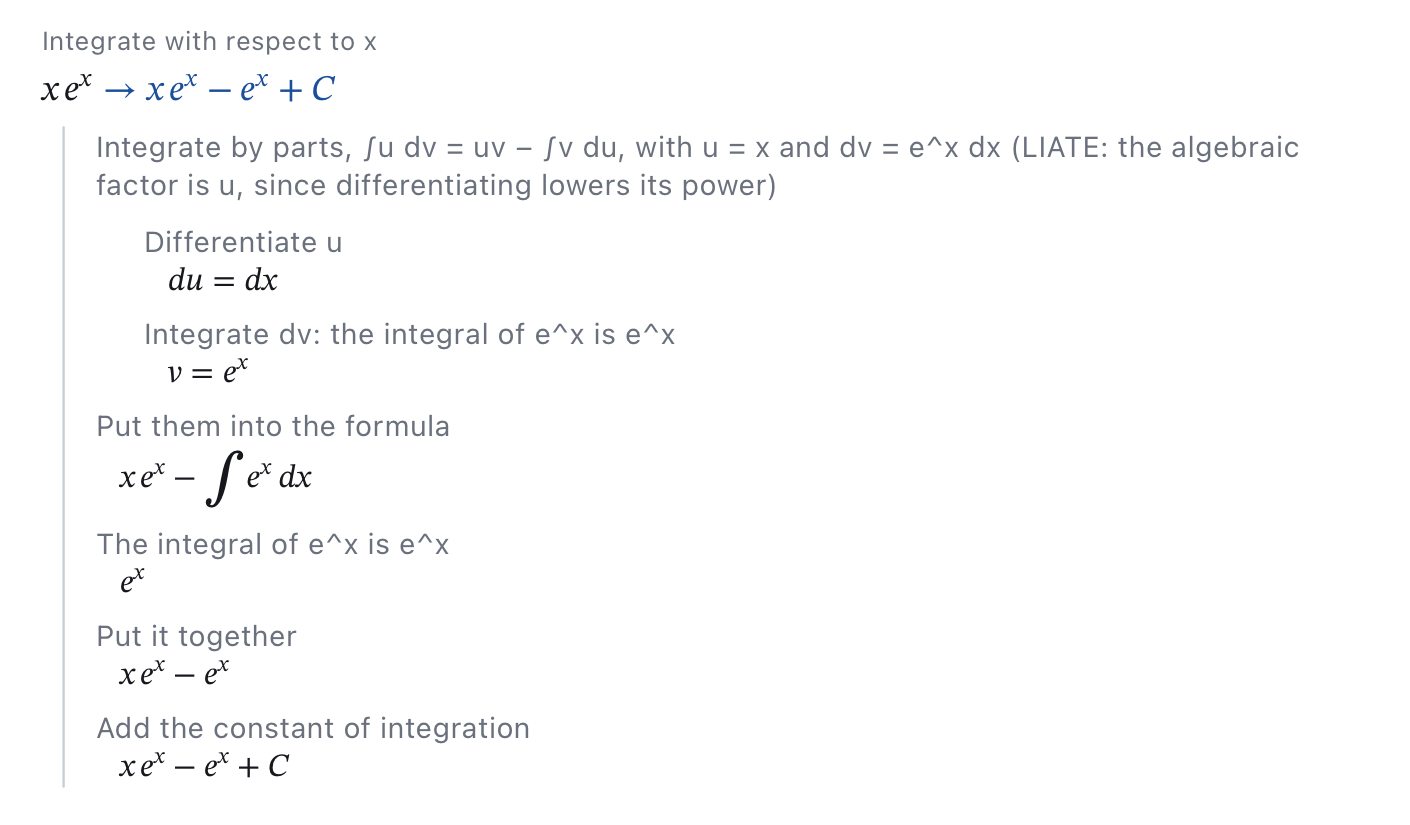
The notebook tries the methods of a calculus course in turn (substitution, parts, partial fractions, the trigonometric substitutions, the half-angle substitution t = tan(x/2)) and names the one that worked:

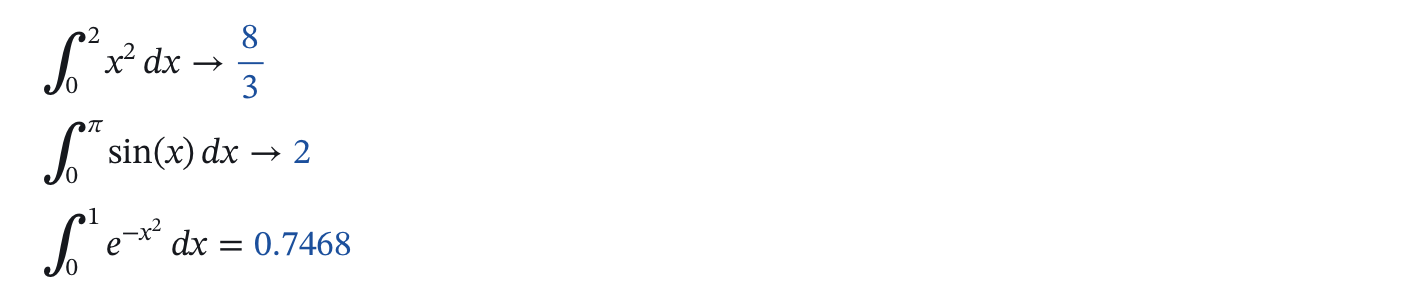
With limits (Cmd+Shift+I is the integral sign; Insert > Definite Integral has the limits), → gives the exact value and = a number, also where there is no antiderivative to write down:
Limits
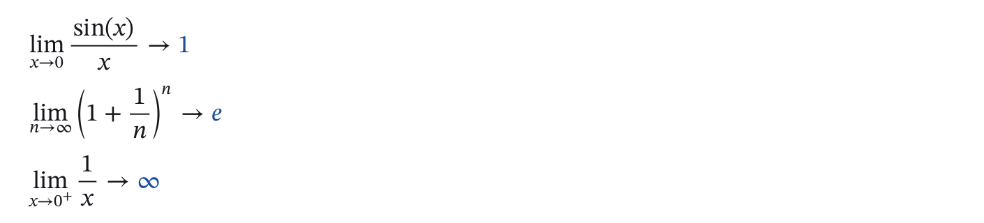
When the answer depends on a letter, the limit comes in cases:

Series and sums
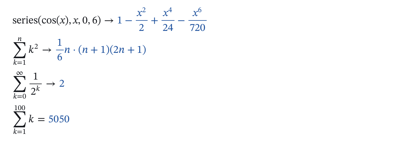
A series can start below the constant term (a Laurent series), and an integral to infinity is a limit: it has a value or it diverges, and the steps say which.

Tangents and curves given by an equation
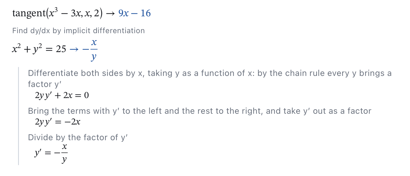
tangent(f, x, a) is the tangent line to y = f(x) at x = a, and implicit(equation, y, x) is dy/dx along the curve an equation in x and y describes. Ask offers both: Tangent line at x = … for an expression (the point is typed in the popup), Find dy/dx (implicit) for an equation in two letters.
Differential equations
Write the equation with primes (an apostrophe after the unknown) and ask: with the caret in it, Ask (Cmd+Return) offers Solve the differential equation for y(x). C₁ and C₂ are the constants of the general solution.
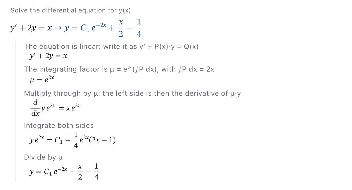
Conditions pin the constants down. In Ask, press Tab and type them with commas between (y(0)=1, y'(0)=0); written out, they follow the variable in dsolve.

Two equations in two unknown functions are a system: a list of equations, the list of unknowns, the variable.

For an equation that has no solution in symbols, odesolve steps a starting value forward in numbers; the Numerical Methods example plots one against the exact solution.
Plots
Plot on the Home tab (Cmd+Option+G), or a kind from the Plot tab, puts a plot under the caret. The caret is then in the plot's own line: type the expression to draw, as a function of x.
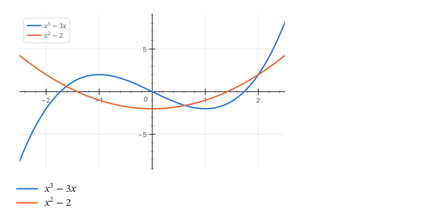
A plot sees the definitions above it, so f(x) can be drawn once f is defined.
Kinds
| Kind | What is drawn | Type |
|---|---|---|
| Graph | y against x | an expression in x |
| Polar | the radius against the angle θ | an expression in θ |
| Parametric | y against x as t runs | two expressions in t |
| Points | data | a list of ys against a list of xs, or a table of two columns |
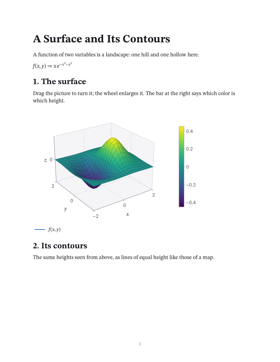
| Surface | the height z over x and y | an expression in x and y |
| Contours | lines of equal height | an expression in x and y |
Traces and the legend
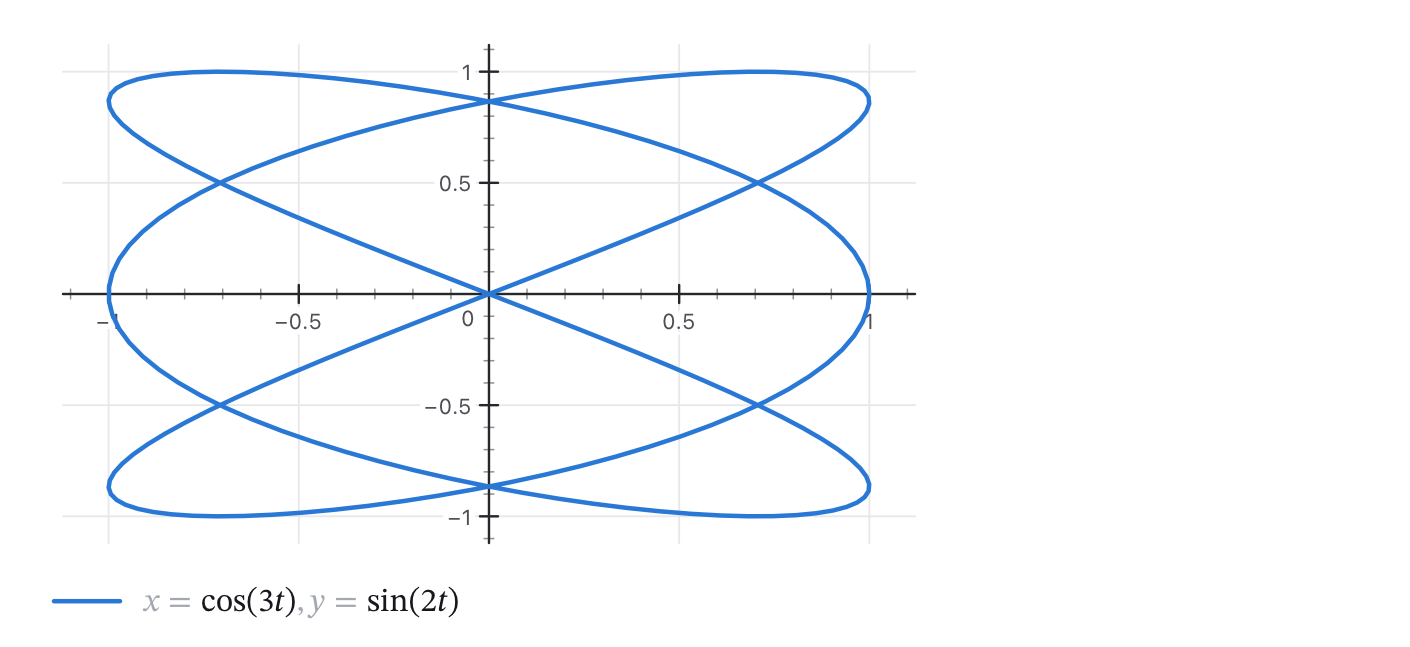
A plot can hold several traces, each with its own line, color and style. Enter in a trace's line starts a new trace under it, and Enter in an empty one ends the list and starts a math region below the plot; Up and Down go from line to line. The Plot tab adds and removes traces too and opens the format panel (Cmd+Shift+F), which has the ranges, titles, labels, grid and legend.
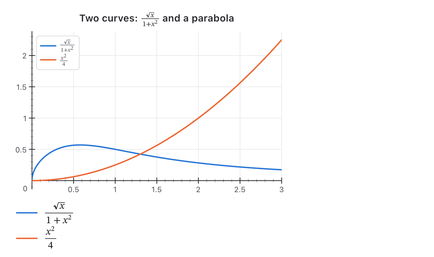
The legend shows each trace as it is written, in real fractions, roots and powers, unless the trace is given a name of its own in the panel. In a name, a title or an axis label, what stands between two $ signs is set as math: Height $h_0 - 1/2 g t^2$.
Marks and shading
Mark (Plot tab, the panel, Format > Plot) puts a dot with its coordinates on the zeros of a graph's curves, on their highest and lowest points, and where two curves cross. They are read off the curve as it was drawn, good to about six digits.
Shade fills the area under the caret's trace down to the x axis, or between it and the next trace, over all that is drawn or between two ends typed in the panel: the picture of a definite integral.
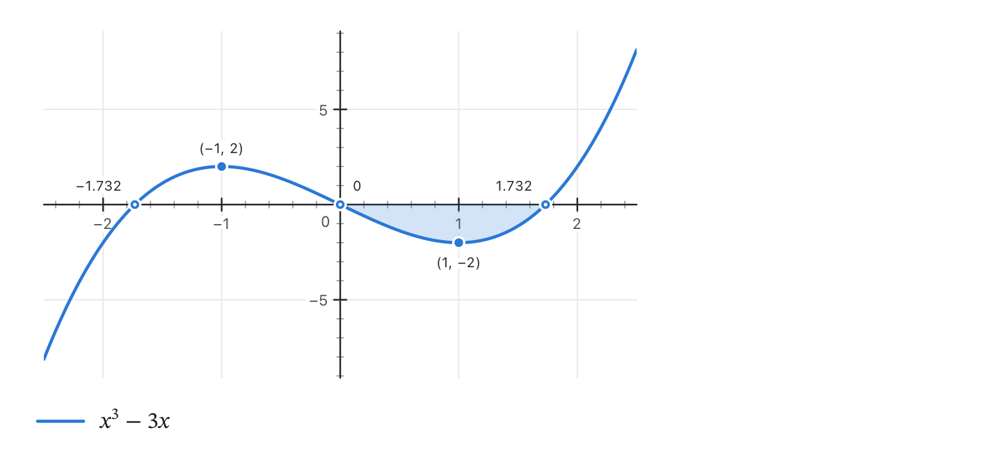
Minor Grid adds the lighter lines between the numbered ones, and Axis Arrows draws the axes through 0 with arrowheads and their names at the tips, as in a textbook.
Surfaces and contours
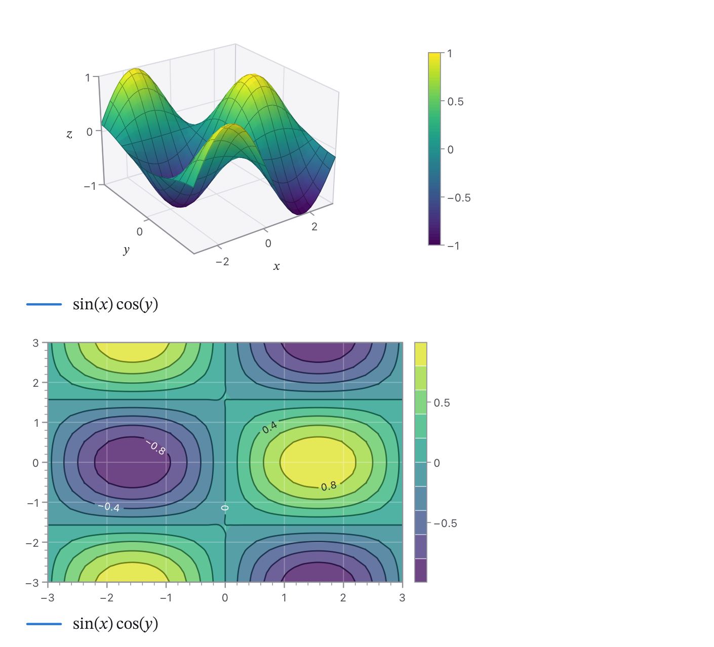
A surface is drawn as a mesh, in the colors of its heights, both, or shaded as if lit from one side; the Color Bar at its right says which color is which height. Contours can be lines or Filled Contours (bands in the colors of their heights), and Contour Levels sets about how many heights are drawn.
The mouse
- Drag the picture to move what it shows; drag a surface to turn it.
- The wheel over the plot the caret is in zooms about the pointer. Everywhere else the wheel scrolls the pages.
- Double-click the picture to go back to the view the plot finds for itself.
- Rest the pointer on a curve to read its coordinates; the corner handle resizes the plot.
Each of these is one step for Undo.
A plot as a picture
Export Picture (Plot tab) saves the caret's plot as a PNG, at 1, 2 or 3 pixels to a point (Picture Sharpness; 2× is the usual for a screen, 3× for print), and Export Picture as PDF as a drawing that stays sharp at any size.
Numbers with units
A plot draws plain numbers. Divide a quantity by its unit to plot it: y(t s)/m is the height in metres at t seconds. The Projectile Motion example does this.
Tables and Pictures
A table of data
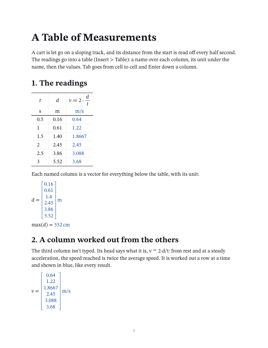
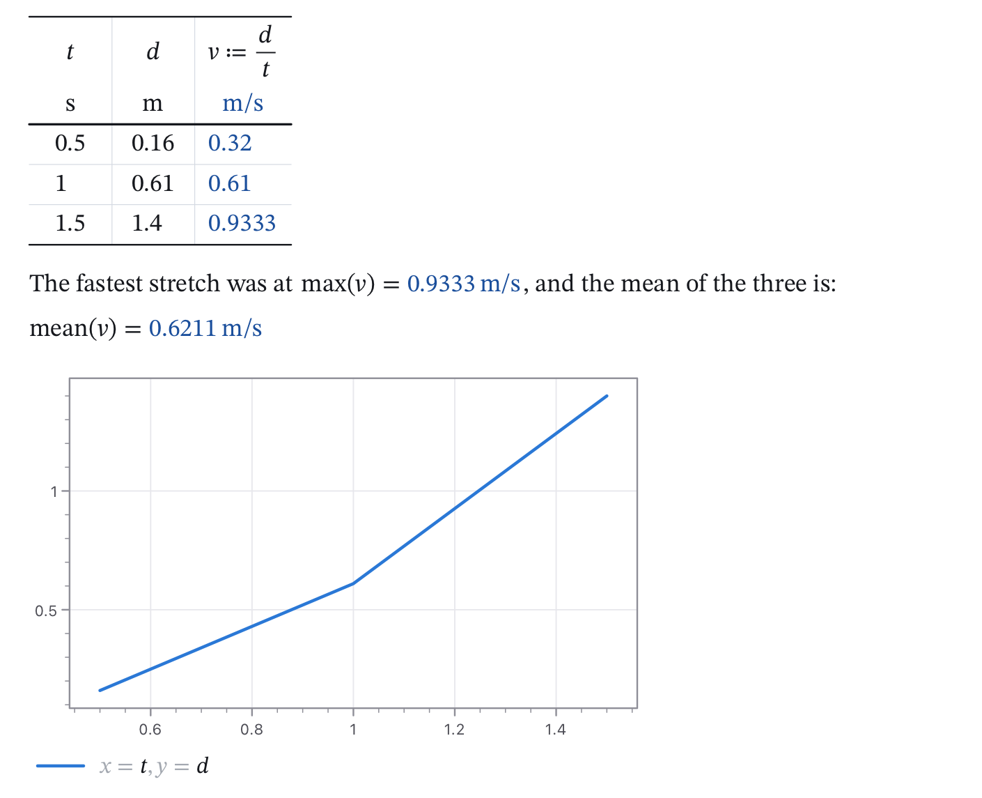
Table on the Insert tab puts a table under the caret: a small grid whose columns are vectors. The first line holds a name for each column (t, F_1, σ), the second its unit, and under them come the values. Every cell is math, so a value can be 2.5, 1/3, 2·10^3 or a formula in names defined above the table.
Below the table each named column is a vector with its unit, like any definition: mean(F)=, F/A=, or the x and y of a plot of kind Points. A column without a name defines nothing.
| Key | What it does |
|---|---|
Tab, Shift+Tab | The next cell, the one before. Tab in the last cell adds a row. |
Enter | One line down; from the last row, a new row. |
| Arrows | From cell to cell at a cell's edges. |
Shift + arrows, or a drag | Selects a rectangle of cells: Copy gives them as text with tabs, Delete empties them. |
Backspace in an empty last row | Takes the row away. |
Escape | Selects the table as a whole (Delete then takes it away). |
A column worked out from the others. Write a head as name ≔ formula, like v ≔ d/t: the column is worked out a row at a time from the other columns and shown in blue. A unit under its head says what to show it in.
Data from elsewhere. Numbers copied in a spreadsheet are pasted with Cmd+V in a cell: they fill the cells from there on, and the table grows to hold them. Paste Data does the same from the menu, and with the caret outside a table makes a new one; Import CSV… brings a file in, Export CSV… writes one. A CSV file dropped on the window becomes a table too.
The right-click menu and Table Tools on the Insert tab have the rest: rows and columns in and out, Sort Rows by the caret's column, Fill Down, and Plot Columns, which makes a plot of two columns. Drag the rule between two columns to make one wider; click it twice to make it fit again.
A cell that can't be worked out gets a red corner, and says what is wrong when the caret is in it. Its column then defines nothing.
Pictures
Picture on the Insert tab puts a PNG or JPEG file on the page; so does dropping the file on the window. The picture is kept inside the notebook (up to 8 MB a picture), so the notebook can be sent as one file.
- Click a picture to select it; drag the handle at its corner to resize it. It keeps its shape unless Shift is held.
- Click it twice, or right-click and choose Caption…, to write a line under it.
- The alignment buttons put it left, in the middle or right. Delete takes a selected picture away.
Sliders and Controls
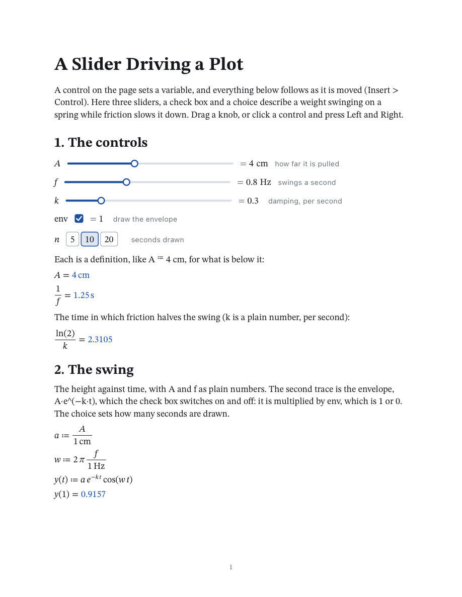
A control is a definition you move with the mouse. Control on the Insert tab puts one under the caret: a slider, a number box, a check box or a choice. Type the name of the variable it sets (a, F_max), press Tab, and type a unit if it has one. From there down the name has the control's value, exactly as after a ≔ 2.5 kN, and every result and plot that uses it follows when the control moves.
| Control | What it gives |
|---|---|
| Slider | A value between its lowest and its highest, in steps. |
| Number box | The same, with two small arrows to step it. |
| Check box | 1 when ticked, 0 when not: multiply by it to switch something on and off. |
| Choice | The value of the button that is taken. The choices are math: 5, 200 GPa, a name defined above. |
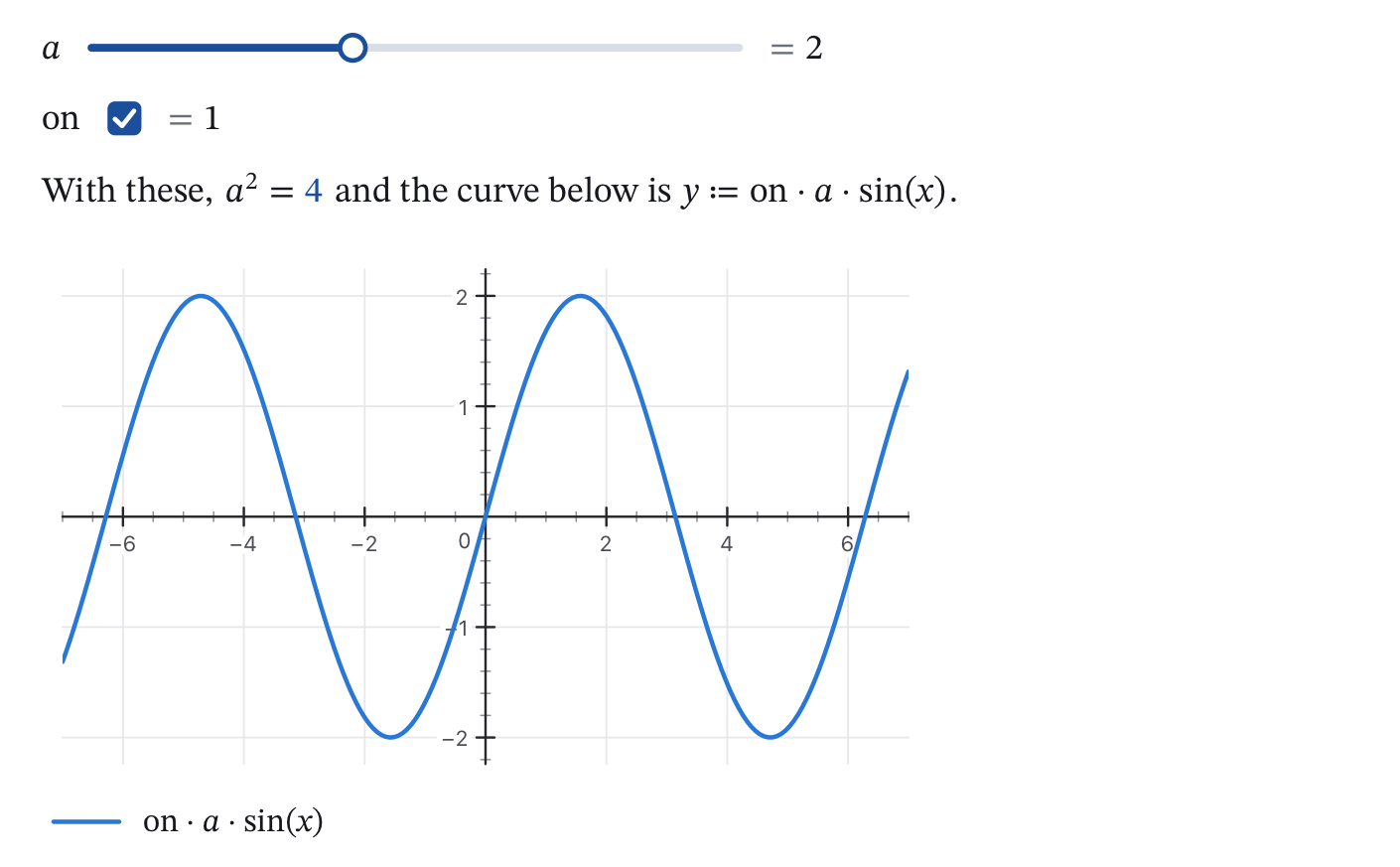
Moving it
- Drag a slider's knob, or press anywhere on its track: the notebook follows while the mouse moves. The whole drag is one step for Undo.
- Click a control to select it; then
LeftandRightnudge it a step,HomeandEndgo to its limits, andSpaceswitches a check box. - Click a slider's or a number box's value twice to type an exact one. It is read as math (
1/3,2π) and taken as it is, off the steps. - The round button right of a selected slider sweeps it from its lowest value to its highest in four seconds. Any key or click stops it.
Setting it up
Format Control… (in the right-click menu and in Insert > Control) opens the Control panel: the kind, the lowest and highest value, the step, the width on the page and a caption beside it. Click a line of the panel to change it. The name and the unit are typed on the page; Tab goes between them, and through the choices of a choice. A double click on a choice puts the caret in it.
To and from a definition
Turn into a Slider makes a slider of a math region that defines a name as a plain number, with a unit or without: L ≔ 4 m becomes a slider from 0 to 10 m. Turn into Math makes the definition of a control again. In exports a control is written as its definition, a = 2.5 kN.
Programming
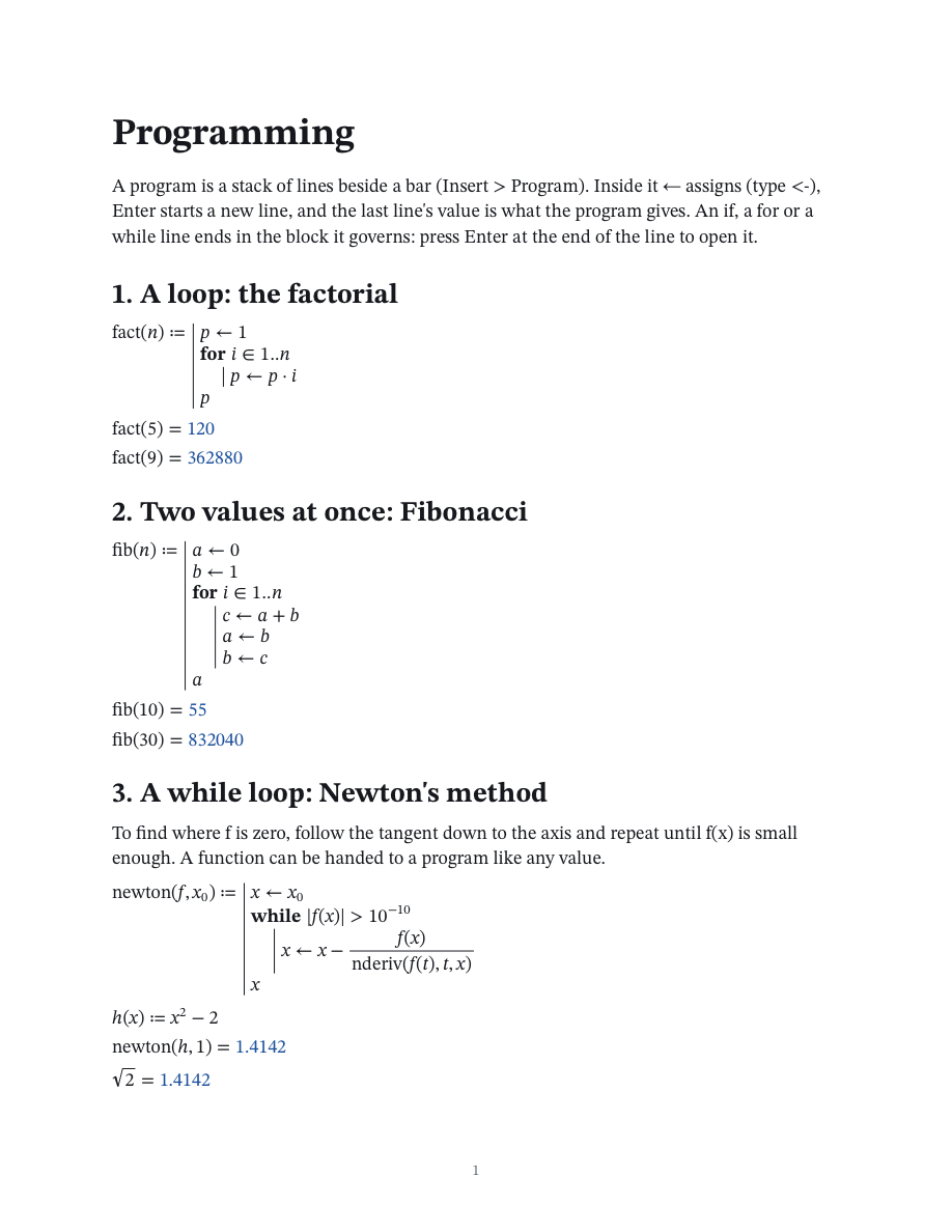
A program is several lines beside a bar, worked from the top; the value of its last line is the value of the program. Insert > Program starts one, usually as the body of a function.
| In a program | Typed | Means |
|---|---|---|
| ← | <- | Gives a name a value inside the program. |
Enter | A new line. At the end of an if, for or while line it opens the block under it; on an empty last line of a block it leaves the block. | |
if … else if … else | the words | Lines that choose. |
for i ∈ 1..n | for i in 1..n | A loop over a range or a list. |
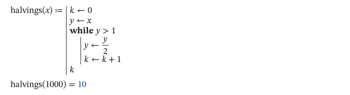
while | the word | A loop while something holds. |
return, break, continue | the words | Leave the program, leave the loop, go to the loop's next turn. |
| Type | You get | |
|---|---|---|
| Insert > Programs<-0Enters+1 | 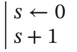 | A program starts with one line: <- is ←, and Enter adds another line under it. |
A loop

An if
A while
Cases
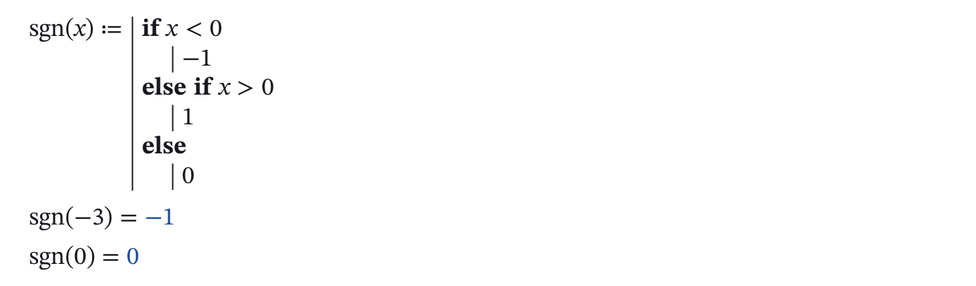
For a function that is one thing here and another there, cases (Insert > Cases) is shorter than a program. An empty last condition means otherwise.
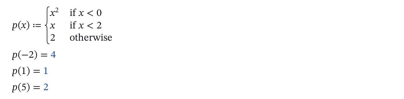
Conditions use <, <=, >, >=, =, !=, and the words and, or, not. A function can be passed to another function by its name; the Programming example has Newton's method written that way.
Working in MathPad
Panels and Tools
Everything here is also in the menus and on the ribbon; the keys are the quick way.
Ask
Cmd+Return in a math region opens a small list of what can be asked of it, only what makes sense for what is written and the most useful first: for an expression Simplify, Differentiate, Integrate and the rest, with its tangent line; for an equation Solve for each unknown, in symbols or in numbers, and dy/dx along its curve; for an equation with a derivative in it (y′) its solution as a differential equation; for a matrix its determinant, inverse, eigenvalues, eigenvectors, row-reduced form and transpose. Type a few letters to narrow the list, choose with the arrows and press Return. Some questions have a line of their own under the list: a limit the point the variable goes to and the side, a series its point and how far it goes, a derivative its order, an integral its two limits (left empty for the antiderivative), a tangent its point, a differential equation its conditions (y(0)=1, y'(0)=0, left empty for the general solution). Tab goes to what is typed there, and Left and Right change the order or the side.
Quick Insert and the Palette
Cmd+K opens Quick Insert at the caret: type a few letters (int, sq, alpha, kPa) to find a template, a symbol, a function or a unit by its name, and Return puts it in. The Palette (Cmd+Shift+P) shows the same things at the side of the pages, in sections that fold: click one to put it in at the caret, and rest the mouse on it to see what it is.
The side panels
One panel shows at a time, at the right of the pages; the View tab and the View menu have them all.
| Panel | Keys | Shows |
|---|---|---|
| Palette | Cmd+Shift+P | Templates, symbols, functions and units to put in. |
| Variables | Cmd+Shift+V | Every name the notebook defines with its value, in the units it was given in; a click goes to the definition. A name that is a unit's name too is marked also a unit (see Units). Under them, how the notebook reads angles and shows results. |
| Plot | Cmd+Shift+F | The plot the caret is in: its kind, titles, ranges, axes, traces and size. |
| Notebook | How many pages, regions and words there are, and the list of problems. |
Problems
When a region can't be worked out, the status bar counts the problems; a click on the count opens the Notebook panel with the list, and a click on a problem there goes to its region. Cmd+' goes to the next one.
Find and Replace
Cmd+F opens the find bar over the top of the pages, Cmd+Option+F with the line for replacing. What is typed is looked for in text and in math as it is written on one line (x^2, sqrt(); Cmd+G and Cmd+Shift+G go to the next and the previous place. Aa minds capitals, Word takes whole words only, and the last three choose where to look. Escape closes the bar.
Number Format and Steps Options
Number Format (Math tab) sets how many digits the caret's region shows, and for the whole notebook the digits after the point and from where numbers are written with a power of ten. Steps Options shows or hides the working of every region at once, copies a region's working as text, and says how much working the notebook shows: all of it, or the main line only, without the working of the parts.
Page Setup and Notebook Settings
Page Setup (File menu, Layout tab) has the paper's size and orientation, the margins, the ruling, and the header and footer, with a small picture of the page. Notebook Settings (Cmd+,) has the notebook's title and author, how numbers and angles are shown, whether results get a prefix chosen for them (kN, MPa, kW), and the fonts. Both can make their choices the default for new notebooks. A page break is Cmd+Shift+Return.
Files and Export
Notebooks
A notebook is saved as a .mathpad file (Cmd+S; Cmd+Shift+S for a copy under another name). What is saved is what you wrote; results are worked out again when the file is opened.
Each notebook you open or start (Cmd+O, Cmd+N) gets a tab of its own above the ribbon. Cmd+W closes the one that shows, and asks first when it has unsaved changes. The File menu remembers the files opened lately.
While you work, a copy of every unsaved notebook is kept every half minute. If MathPad should close unexpectedly, it offers to bring them back the next time it starts.
Bringing text in
File > Import Text (or opening a .txt or .md file) makes a new notebook from plain text or Markdown.
Export
| Export | For |
|---|---|
PDF (Cmd+Shift+E) | The pages exactly as they look. |
| LaTeX | A .tex file with the math as LaTeX, units upright. |
| Markdown | Text with the math in it, and the plots as pictures next to the file. |
| Web Page | One .html file to open in a browser. |
| Plain Text | The math as one line of text each. |
Print (Cmd+P) sends the pages to the printer.
The paper
The Layout tab sets the paper's size, its margins and orientation, a header and page numbers, and whether the page is plain, lined or squared. View has the zoom (Cmd+=, Cmd+-, Cmd+0 for actual size, Cmd+9 for the page's width).
The clipboard
Copied math goes to the clipboard as one line of text as well, so it can be pasted into other programs; text pasted into a math region from another program is typed in, so 1/2 becomes a real fraction.
Keyboard Shortcuts
Every command that has keys, by menu. The keys for typing math are in Typing Math.
File
| Command | Keys |
|---|---|
| New | Cmd+N |
| Open | Cmd+O |
| Close Notebook | Cmd+W |
| Save | Cmd+S |
| Save As | Cmd+Shift+S |
| Export as PDF | Cmd+Shift+E |
Cmd+P |
Edit
| Command | Keys |
|---|---|
| Undo | Cmd+Z |
| Redo | Cmd+Shift+Z |
| Cut | Cmd+X |
| Copy | Cmd+C |
| Paste | Cmd+V |
| Select All | Cmd+A |
| Select Region | Cmd+Shift+A |
| Find | Cmd+F |
| Find Next | Cmd+G |
| Find Previous | Cmd+Shift+G |
| Replace | Cmd+Option+F |
Region
| Command | Keys |
|---|---|
| Math | Cmd+Shift+M |
| Text | Cmd+Shift+T |
| Plot | Cmd+Option+G |
| Delete Region | Cmd+Shift+Backspace |
| Move Region Up | Cmd+Option+Up |
| Move Region Down | Cmd+Option+Down |
| Duplicate Region | Cmd+D |
| Leave Out of the Working | Cmd+Shift+O |
Insert
| Command | Keys |
|---|---|
| Page Break | Cmd+Shift+Enter |
| Square Root | Cmd+Shift+Q |
| Sum | Cmd+Shift+U |
| Integral | Cmd+Shift+I |
| Derivative | Cmd+Shift+D |
| Matrix | Ctrl+M |
| Quick Insert | Cmd+K |
| Inline Math | Ctrl+= |
| Reference | Cmd+Option+R |
Math
| Command | Keys |
|---|---|
| Show Steps | Cmd+Shift+W |
| More Digits | Cmd+Shift+. |
| Fewer Digits | Cmd+Shift+, |
| Work Out Again | Cmd+R |
| Solve | Cmd+E |
| Simplify | Cmd+Shift+Y |
| Evaluate | Cmd+Shift+N |
| Ask | Cmd+Enter |
| Number Equation | Cmd+Option+N |
Format
| Command | Keys |
|---|---|
| Bold | Cmd+B |
| Italic | Cmd+I |
| Underline | Cmd+U |
| Fixed Width | Cmd+Shift+K |
| Highlight | Cmd+Shift+H |
| Align Left | Cmd+Shift+L |
| Center | Cmd+Shift+C |
| Align Right | Cmd+Shift+R |
| Increase Indent | Cmd+] |
| Decrease Indent | Cmd+[ |
| Body | Cmd+Option+0 |
| Title | Cmd+Option+1 |
| Heading 1 | Cmd+Option+2 |
| Heading 2 | Cmd+Option+3 |
| Heading 3 | Cmd+Option+4 |
View
| Command | Keys |
|---|---|
| Zoom In | Cmd+= |
| Zoom Out | Cmd+- |
| Actual Size | Cmd+0 |
| Page Width | Cmd+9 |
| Palette | Cmd+Shift+P |
| Variables | Cmd+Shift+V |
Plot
| Command | Keys |
|---|---|
| Format Plot | Cmd+Shift+F |
Layout
| Command | Keys |
|---|---|
| Notebook Settings | Cmd+, |
| Next Problem | Cmd+' |
Help
| Command | Keys |
|---|---|
| MathPad Guide | Cmd+Shift+/ |
In math
| Key | What it does |
|---|---|
/ | A fraction; after the units of a number (9.81 m), the stroke of m/s² |
^ | A power; x^(n+1) for more than one thing in it |
_ | A subscript |
+ - * / = , ) | After a simple power or subscript: out of it, then the sign |
[ | An index, or a list |
\ | A square root |
: | ≔ (define) |
-> | → (in symbols) |
Space | Out of a structure; between names, times |
Tab | The next empty place |
Enter | A new region; a new line of a program; a new trace of a plot |
" | Text: in an empty region a text region, in math a string |
Reference
Functions Reference
Every function MathPad knows, by group. Names are in small letters. Type a name and its bracket, or pick it from the palette (View > Palette).
Elementary
| Function | What it gives |
|---|---|
sin(x) | The sine of an angle. |
cos(x) | The cosine of an angle. |
tan(x) | The tangent of an angle. |
cot(x) | The cotangent of an angle: cos(x)/sin(x). |
sec(x) | The secant of an angle: 1/cos(x). |
csc(x) | The cosecant of an angle: 1/sin(x). |
asin(x) | The angle whose sine is x. |
acos(x) | The angle whose cosine is x. |
atan(x) | The angle whose tangent is x. |
acot(x) | The angle whose cotangent is x. |
asec(x) | The angle whose secant is x. |
acsc(x) | The angle whose cosecant is x. |
atan2(y, x) | The angle from the x axis to the point (x, y). |
sinh(x) | The hyperbolic sine. |
cosh(x) | The hyperbolic cosine. |
tanh(x) | The hyperbolic tangent. |
coth(x) | The hyperbolic cotangent. |
sech(x) | The hyperbolic secant. |
csch(x) | The hyperbolic cosecant. |
asinh(x) | The inverse hyperbolic sine. |
acosh(x) | The inverse hyperbolic cosine. |
atanh(x) | The inverse hyperbolic tangent. |
exp(x) | e to the power x. |
ln(x) | The natural logarithm. |
log(x) or log(x, b) | The logarithm to base 10, or to base b. |
log2(x) | The logarithm to base 2. |
log10(x) | The logarithm to base 10. |
sqrt(x) | The square root. |
cbrt(x) | The cube root. |
root(x, n) or root(f, x, a, b) | The n-th root of x; or, with four values, where f is zero for x between a and b. |
abs(x) | The size of a number without its sign; of a complex number, its modulus. |
sign(x) | −1, 0 or 1 as x is negative, zero or positive. |
floor(x) | x rounded down to a whole number. |
ceil(x) | x rounded up to a whole number. |
round(x) or round(x, n) | x rounded to the nearest whole number, or to n decimals. |
trunc(x) | x without its fraction. |
mod(a, b) | What is left of a after dividing by b. |
gcd(a, b) | The greatest common divisor. |
lcm(a, b) | The least common multiple. |
factorial(n) | n! = 1·2·3·…·n. |
ncr(n, k) | The number of ways to choose k of n things. |
npr(n, k) | The number of ways to arrange k of n things. |
min(a, b, …) | The smallest of the values, or of a list. |
max(a, b, …) | The largest of the values, or of a list. |
re(z) | The real part of a complex number. |
im(z) | The imaginary part of a complex number. |
arg(z) | The angle of a complex number. |
conj(z) | The complex conjugate. |
Statistics and lists
| Function | What it gives |
|---|---|
sum(v) | The values of a list added up. |
mean(v) | The average of a list. |
median(v) | The middle value of a list. |
stdev(v) | The standard deviation of a sample. |
var(v) | The variance of a sample. |
sort(v) | The list in rising order. |
reverse(v) | The list back to front. |
length(v) | How many values a list has. |
last(v) | The last value of a list. |
linspace(a, b, n) | n evenly spaced values from a to b. |
Symbolic
| Function | What it gives |
|---|---|
simplify(e) | The expression in a simpler form. |
expand(e) | Products and powers multiplied out. |
factor(e) | The expression as a product of factors. |
collect(e, x) | Terms gathered by powers of x. |
partfrac(e, x) | A fraction split into partial fractions. |
together(e) | Fractions brought over one denominator. |
substitute(e, x, a) | The expression with a in place of x. |
solve(eq, x) or solve([eqs], [vars]) | The values that satisfy an equation, or a system. |
diff(e, x) or diff(e, x, n) | The derivative with respect to x, or the n-th. |
integrate(e, x) or integrate(e, x, a, b) | The antiderivative, or the integral from a to b. |
limit(e, x, a) | What e approaches as x goes to a. |
series(e, x, a, n) | The Taylor series about a, up to order n. |
dsolve(eq, y, x) | The function y(x) that satisfies a differential equation. |
implicit(eq, y, x) or implicit(eq, y, x, 2) | The slope dy/dx along the curve an equation in x and y gives, or the second derivative. |
tangent(f, x, a) | The tangent line to y = f(x) at x = a. |
Numerical
| Function | What it gives |
|---|---|
nsolve(eq, x, guess) | A solution of an equation near a guess, in numbers. |
polyroots(v) | All roots of the polynomial with coefficients v. |
fsolve([eqs], [vars], [guesses]) | A solution of a system near the guesses. |
nintegrate(f, x, a, b) | The integral from a to b, in numbers. |
nderiv(f, x, a) | The slope of f at x = a, in numbers. |
odesolve(f, y0, t0, t1, n) | Solves y′ = f(t, y) from t0 to t1 in n steps; a matrix of t and y. |
minimize(f, x, guess) | The x near a guess where f is smallest. |
maximize(f, x, guess) | The x near a guess where f is largest. |
interp(xs, ys, x) | The value at x on straight lines through the points. |
spline(xs, ys, x) | The value at x on a smooth curve through the points. |
linfit(xs, ys) | The line that fits the points best: [intercept, slope]. |
polyfit(xs, ys, n) | The polynomial of degree n that fits the points best. |
Matrices
| Function | What it gives |
|---|---|
det(M) | The determinant. |
inv(M) | The inverse matrix. |
transpose(M) | Rows and columns swapped. |
identity(n) | The n by n identity matrix. |
zeros(r, c) | A matrix of zeros. |
ones(r, c) | A matrix of ones. |
rows(M) | How many rows a matrix has. |
cols(M) | How many columns a matrix has. |
rank(M) | The rank of a matrix. |
trace(M) | The sum of the diagonal. |
eigenvalues(M) | The eigenvalues, as a vector. |
eigenvectors(M) | The eigenvectors, as the columns of a matrix. |
lsolve(A, b) | The x for which A·x = b. |
rref(M) | The reduced row echelon form. |
cross(a, b) | The cross product of two vectors. |
dot(a, b) | The dot product of two vectors. |
norm(v) | The length of a vector. |
augment(A, B) | Two matrices side by side. |
stack(A, B) | One matrix on top of another. |
submatrix(M, r1, r2, c1, c2) | Rows r1 to r2 and columns c1 to c2 of a matrix. |
diag(v) | A matrix with v down its diagonal. |
Constants
| Constant | Typed | |
|---|---|---|
| π | pi | The circle number. |
| e | e | The base of natural logarithms. |
| ⅈ | 2i or 2j after a number | The imaginary unit. |
| ∞ | inf | Infinity, for limits and sums. |
Units Reference
Every unit MathPad knows, by what it measures, with what one of it is in SI base units. Type a unit after a number and a Space; type one after a final = to convert. See Units.
Length
| Unit | Name | System | Equals |
|---|---|---|---|
m | metre | SI | 1 m |
pm | picometre | SI | 1e-12 m |
nm | nanometre | SI | 1e-9 m |
μm | micrometre | SI | 1e-6 m |
µm | micrometre | SI | 1e-6 m |
um | micrometre | SI | 1e-6 m |
mm | millimetre | SI | 0.001 m |
cm | centimetre | SI | 0.01 m |
dm | decimetre | SI | 0.1 m |
km | kilometre | SI | 1000 m |
in | inch | US | 0.0254 m |
ft | foot | US | 0.3048 m |
yd | yard | US | 0.9144 m |
mi | mile | US | 1609.344 m |
nmi | nautical mile | SI | 1852 m |
Mass
| Unit | Name | System | Equals |
|---|---|---|---|
g | gram | SI | 0.001 kg |
ng | nanogram | SI | 1e-12 kg |
μg | microgram | SI | 1e-9 kg |
µg | microgram | SI | 1e-9 kg |
ug | microgram | SI | 1e-9 kg |
mg | milligram | SI | 1e-6 kg |
kg | kilogram | SI | 1 kg |
Mg | megagram | SI | 1000 kg |
t | tonne | SI | 1000 kg |
tonne | tonne | SI | 1000 kg |
lb | pound | US | 0.45359237 kg |
lbm | pound | US | 0.45359237 kg |
oz | ounce | US | 0.02834952313 kg |
slug | slug | US | 14.59390294 kg |
ton | short ton | US | 907.18474 kg |
Time
| Unit | Name | System | Equals |
|---|---|---|---|
s | second | SI | 1 s |
ps | picosecond | SI | 1e-12 s |
ns | nanosecond | SI | 1e-9 s |
μs | microsecond | SI | 1e-6 s |
µs | microsecond | SI | 1e-6 s |
us | microsecond | SI | 1e-6 s |
ms | millisecond | SI | 0.001 s |
min | minute | SI | 60 s |
hr | hour | SI | 3600 s |
h | hour | SI | 3600 s |
day | day | SI | 86400 s |
wk | week | SI | 604800 s |
yr | year | SI | 31557600 s |
Electric Current
| Unit | Name | System | Equals |
|---|---|---|---|
A | ampere | SI | 1 A |
nA | nanoampere | SI | 1e-9 A |
μA | microampere | SI | 1e-6 A |
µA | microampere | SI | 1e-6 A |
uA | microampere | SI | 1e-6 A |
mA | milliampere | SI | 0.001 A |
kA | kiloampere | SI | 1000 A |
Temperature
| Unit | Name | System | Equals |
|---|---|---|---|
K | kelvin | SI | 1 K |
mK | millikelvin | SI | 0.001 K |
°C | degree Celsius | SI | 1 K |
degC | degree Celsius | SI | 1 K |
°F | degree Fahrenheit | US | 0.5555555556 K |
degF | degree Fahrenheit | US | 0.5555555556 K |
°R | degree Rankine | US | 0.5555555556 K |
Δ°C | Celsius degree (a difference) | SI | 1 K |
Δ°F | Fahrenheit degree (a difference) | US | 0.5555555556 K |
Amount Of Substance
| Unit | Name | System | Equals |
|---|---|---|---|
mol | mole | SI | 1 mol |
μmol | micromole | SI | 1e-6 mol |
µmol | micromole | SI | 1e-6 mol |
umol | micromole | SI | 1e-6 mol |
mmol | millimole | SI | 0.001 mol |
kmol | kilomole | SI | 1000 mol |
Luminous Intensity
| Unit | Name | System | Equals |
|---|---|---|---|
cd | candela | SI | 1 cd |
Angle
| Unit | Name | System | Equals |
|---|---|---|---|
rad | radian | SI | 1 rad |
mrad | milliradian | SI | 0.001 rad |
deg | degree | SI | 0.01745329252 rad |
° | degree | SI | 0.01745329252 rad |
rev | revolution | SI | 6.283185307 rad |
Angular Speed
| Unit | Name | System | Equals |
|---|---|---|---|
rpm | revolution per minute | SI | 0.1047197551 1/s |
Force
| Unit | Name | System | Equals |
|---|---|---|---|
N | newton | SI | 1 N |
μN | micronewton | SI | 1e-6 N |
µN | micronewton | SI | 1e-6 N |
uN | micronewton | SI | 1e-6 N |
mN | millinewton | SI | 0.001 N |
kN | kilonewton | SI | 1000 N |
MN | meganewton | SI | 1000000 N |
GN | giganewton | SI | 1000000000 N |
kgf | kilogram-force | SI | 9.80665 N |
dyn | dyne | SI | 1e-5 N |
lbf | pound-force | US | 4.448221615 N |
kip | kip (1000 pounds-force) | US | 4448.221615 N |
tonf | short ton-force | US | 8896.443231 N |
Pressure
| Unit | Name | System | Equals |
|---|---|---|---|
Pa | pascal | SI | 1 Pa |
mPa | millipascal | SI | 0.001 Pa |
hPa | hectopascal | SI | 100 Pa |
kPa | kilopascal | SI | 1000 Pa |
MPa | megapascal | SI | 1000000 Pa |
GPa | gigapascal | SI | 1000000000 Pa |
bar | bar | SI | 100000 Pa |
mbar | millibar | SI | 100 Pa |
atm | atmosphere | SI | 101325 Pa |
torr | torr | SI | 133.3223684 Pa |
mmHg | millimetre of mercury | SI | 133.3223874 Pa |
psi | pound per square inch | US | 6894.757293 Pa |
ksi | kip per square inch | US | 6894757.293 Pa |
psf | pound per square foot | US | 47.88025898 Pa |
ksf | kip per square foot | US | 47880.25898 Pa |
Energy
| Unit | Name | System | Equals |
|---|---|---|---|
J | joule | SI | 1 J |
mJ | millijoule | SI | 0.001 J |
kJ | kilojoule | SI | 1000 J |
MJ | megajoule | SI | 1000000 J |
GJ | gigajoule | SI | 1000000000 J |
Wh | watt-hour | SI | 3600 J |
kWh | kilowatt-hour | SI | 3600000 J |
MWh | megawatt-hour | SI | 3600000000 J |
GWh | gigawatt-hour | SI | 3600000000000 J |
cal | calorie | SI | 4.184 J |
kcal | kilocalorie | SI | 4184 J |
eV | electronvolt | SI | 1.602176634e-19 J |
keV | kiloelectronvolt | SI | 1.602176634e-16 J |
MeV | megaelectronvolt | SI | 1.602176634e-13 J |
GeV | gigaelectronvolt | SI | 1.602176634e-10 J |
BTU | British thermal unit | US | 1055.055853 J |
Power
| Unit | Name | System | Equals |
|---|---|---|---|
W | watt | SI | 1 W |
μW | microwatt | SI | 1e-6 W |
µW | microwatt | SI | 1e-6 W |
uW | microwatt | SI | 1e-6 W |
mW | milliwatt | SI | 0.001 W |
kW | kilowatt | SI | 1000 W |
MW | megawatt | SI | 1000000 W |
GW | gigawatt | SI | 1000000000 W |
hp | horsepower | US | 745.6998716 W |
Electric Potential
| Unit | Name | System | Equals |
|---|---|---|---|
V | volt | SI | 1 V |
μV | microvolt | SI | 1e-6 V |
µV | microvolt | SI | 1e-6 V |
uV | microvolt | SI | 1e-6 V |
mV | millivolt | SI | 0.001 V |
kV | kilovolt | SI | 1000 V |
MV | megavolt | SI | 1000000 V |
Electric Resistance
| Unit | Name | System | Equals |
|---|---|---|---|
Ω | ohm | SI | 1 Ω |
mΩ | milliohm | SI | 0.001 Ω |
kΩ | kiloohm | SI | 1000 Ω |
MΩ | megaohm | SI | 1000000 Ω |
GΩ | gigaohm | SI | 1000000000 Ω |
ohm | ohm | SI | 1 Ω |
kohm | kiloohm | SI | 1000 Ω |
Mohm | megaohm | SI | 1000000 Ω |
Capacitance
| Unit | Name | System | Equals |
|---|---|---|---|
F | farad | SI | 1 F |
pF | picofarad | SI | 1e-12 F |
nF | nanofarad | SI | 1e-9 F |
μF | microfarad | SI | 1e-6 F |
µF | microfarad | SI | 1e-6 F |
uF | microfarad | SI | 1e-6 F |
mF | millifarad | SI | 0.001 F |
Inductance
| Unit | Name | System | Equals |
|---|---|---|---|
H | henry | SI | 1 H |
nH | nanohenry | SI | 1e-9 H |
μH | microhenry | SI | 1e-6 H |
µH | microhenry | SI | 1e-6 H |
uH | microhenry | SI | 1e-6 H |
mH | millihenry | SI | 0.001 H |
Electric Charge
| Unit | Name | System | Equals |
|---|---|---|---|
C | coulomb | SI | 1 C |
nC | nanocoulomb | SI | 1e-9 C |
μC | microcoulomb | SI | 1e-6 C |
µC | microcoulomb | SI | 1e-6 C |
uC | microcoulomb | SI | 1e-6 C |
mC | millicoulomb | SI | 0.001 C |
Electric Conductance
| Unit | Name | System | Equals |
|---|---|---|---|
S | siemens | SI | 1 1/Ω |
μS | microsiemens | SI | 1e-6 1/Ω |
µS | microsiemens | SI | 1e-6 1/Ω |
uS | microsiemens | SI | 1e-6 1/Ω |
mS | millisiemens | SI | 0.001 1/Ω |
Magnetic Flux Density
| Unit | Name | System | Equals |
|---|---|---|---|
T | tesla | SI | 1 N/(m·A) |
μT | microtesla | SI | 1e-6 N/(m·A) |
µT | microtesla | SI | 1e-6 N/(m·A) |
uT | microtesla | SI | 1e-6 N/(m·A) |
mT | millitesla | SI | 0.001 N/(m·A) |
Magnetic Flux
| Unit | Name | System | Equals |
|---|---|---|---|
Wb | weber | SI | 1 J/A |
Frequency
| Unit | Name | System | Equals |
|---|---|---|---|
Hz | hertz | SI | 1 1/s |
kHz | kilohertz | SI | 1000 1/s |
MHz | megahertz | SI | 1000000 1/s |
GHz | gigahertz | SI | 1000000000 1/s |
Volume
| Unit | Name | System | Equals |
|---|---|---|---|
L | litre | SI | 0.001 m³ |
μL | microlitre | SI | 1e-9 m³ |
µL | microlitre | SI | 1e-9 m³ |
uL | microlitre | SI | 1e-9 m³ |
mL | millilitre | SI | 1e-6 m³ |
cL | centilitre | SI | 1e-5 m³ |
dL | decilitre | SI | 0.0001 m³ |
gal | US gallon | US | 0.003785411784 m³ |
qt | US quart | US | 0.000946352946 m³ |
floz | US fluid ounce | US | 2.957352956e-5 m³ |
Area
| Unit | Name | System | Equals |
|---|---|---|---|
ha | hectare | SI | 10000 m² |
acre | acre | US | 4046.856422 m² |
Speed
| Unit | Name | System | Equals |
|---|---|---|---|
mph | mile per hour | US | 0.44704 m/s |
kph | kilometre per hour | SI | 0.2777777778 m/s |
knot | knot | SI | 0.5144444444 m/s |
Examples
The example notebooks
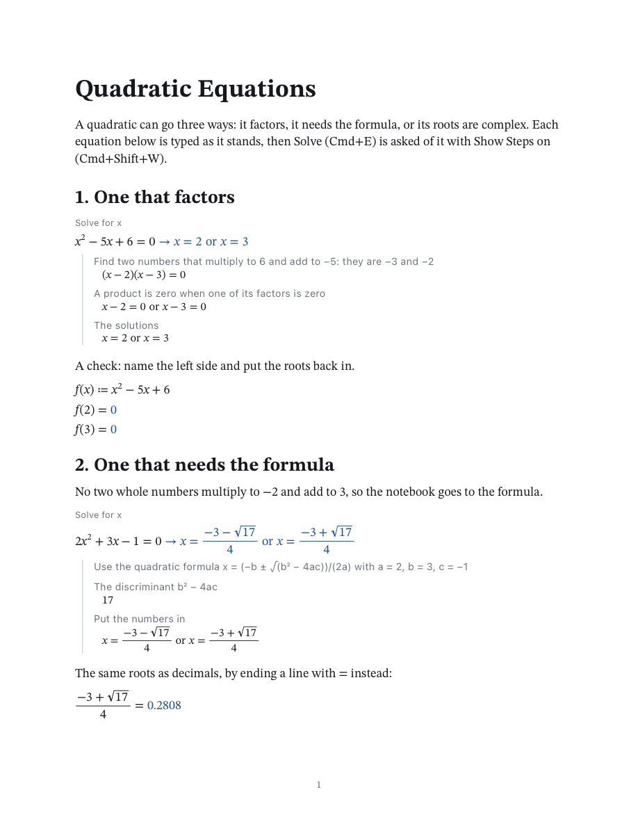
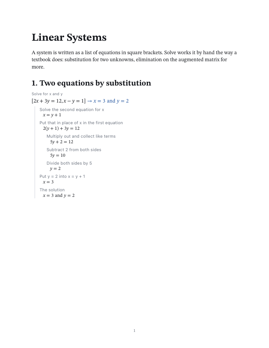
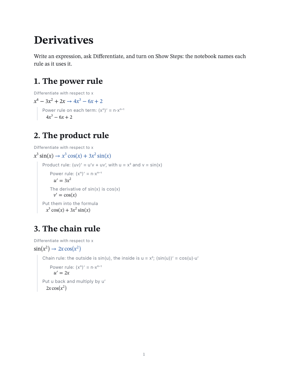
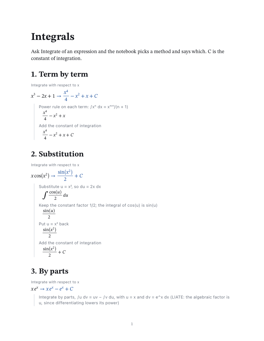
Each opens from Help > Examples (or the gallery) as a new notebook, ready to change: alter a number and everything below it follows. Here is the first page of each.